Optimizing Julia code: Improving the performance of adaptive mesh refinement with p4est in Trixi.jl

In this blog post, I would like to share some experiences with writing efficient code in Julia, my favorite programming language so far. This blog post is not designed as an introduction to Julia in general or the numerical methods we use; I will also not necessarily introduce all concepts in a pedagogically optimal way. Instead, I would like to walk you through the steps I have taken when working on a concrete performance problem in Julia. In particular, we will focus on Issue #627 in Trixi.jl, a framework of high-order methods for hyperbolic conservation laws.

Trixi.jl is an open source project with several contributors. In particular, the code enabling adaptive mesh refinement using the great C library p4est in Trixi.jl was mainly written by Erik Faulhaber under the supervision of Michael Schlottke-Lakemper (and me, partially).

You should not understand this post as some form of criticism like “we need to optimize their code since it was too slow”. I prefer developing in Julia by following the two steps

1. Make it work
2. Make it fast

Erik Faulhaber has done a really great job at the first step. Note that this first step includes adding tests and continuous integration, so that we can refactor or rewrite code later without worrying about introducing bugs or regressions. This step is absolutely necessary for any code you want to rely on! Armed with this background, we can take the next step and improve the performance.

Step 0: Start a Julia REPL and load some packages

All results shown below are obtained using Julia v1.6.1 and command line flags julia --threads=1 --check-bounds=no. You can find a complete set of commits and all the code in the branch hr/blog_p4est_performance in my fork of Trixi.jl and the associated PR #638.

Let’s start by loading some packages.

julia> using BenchmarkHistograms, ProfileView; using Revise, Trixi

BenchmarkHistograms.jl is basically a wrapper of BenchmarkTools.jl that prints benchmark results as histograms, providing more detailed information about the performance of a piece of code. ProfileView.jl allows us to profile code and visualize the results. Finally, Revise.jl makes editing Julia packages much more comfortable by re-loading modified code on the fly. If you’re not familiar with these packages, I highly recommend taking a look at them.

Next, we run some code as described in Issue #627. At first, we perform an adaptive mesh refinement (AMR) simulation on the TreeMesh in Trixi.jl. The result shown below is obtained after running the command twice to exclude compilation time. I have removed parts of the output that are not interesting for the current task of optimizing the AMR step.

julia> trixi_include(joinpath(examples_dir(), "2d", "elixir_advection_amr.jl"))
[...]
 ─────────────────────────────────────────────────────────────────────────────────────
               Trixi.jl                       Time                   Allocations
                                      ──────────────────────   ───────────────────────
           Tot / % measured:               107ms / 92.9%           15.6MiB / 99.2%

 Section                      ncalls     time   %tot     avg     alloc   %tot      avg
 ─────────────────────────────────────────────────────────────────────────────────────
 rhs!                          1.60k   59.1ms  59.3%  36.9μs    586KiB  3.69%     375B
[...]
 AMR                              63   29.1ms  29.2%   461μs   13.2MiB  85.4%   215KiB
   refine                         63   18.6ms  18.7%   296μs   5.57MiB  36.0%  90.6KiB
     solver                       63   15.9ms  16.0%   253μs   5.06MiB  32.6%  82.2KiB
     mesh                         63   2.18ms  2.19%  34.6μs    459KiB  2.89%  7.28KiB
       refine_unbalanced!         63   1.94ms  1.95%  30.9μs   8.59KiB  0.05%     140B
       ~mesh~                     63    186μs  0.19%  2.95μs    348KiB  2.20%  5.53KiB
       rebalance!                 63   50.9μs  0.05%   807ns    102KiB  0.64%  1.62KiB
     ~refine~                     63    536μs  0.54%  8.50μs   69.2KiB  0.44%  1.10KiB
   coarsen                        63   8.17ms  8.20%   130μs   7.14MiB  46.1%   116KiB
     solver                       63   4.95ms  4.96%  78.5μs   5.18MiB  33.5%  84.2KiB
     mesh                         63   2.48ms  2.49%  39.3μs    302KiB  1.90%  4.79KiB
     ~coarsen~                    63    750μs  0.75%  11.9μs   1.67MiB  10.8%  27.1KiB
   indicator                      63   1.83ms  1.84%  29.1μs     0.00B  0.00%    0.00B
   ~AMR~                          63    415μs  0.42%  6.58μs    516KiB  3.26%  8.20KiB
[...]
 initial condition AMR             1    733μs  0.74%   733μs    484KiB  3.05%   484KiB
   AMR                             3    531μs  0.53%   177μs    484KiB  3.05%   161KiB
     refine                        3    458μs  0.46%   153μs    354KiB  2.23%   118KiB
       mesh                        2    248μs  0.25%   124μs   21.8KiB  0.14%  10.9KiB
         refine_unbalanced!        2    235μs  0.24%   117μs      672B  0.00%     336B
         ~mesh~                    2   11.2μs  0.01%  5.61μs   16.2KiB  0.10%  8.10KiB
         rebalance!                2   1.44μs  0.00%   719ns   4.94KiB  0.03%  2.47KiB
       solver                      2    192μs  0.19%  96.0μs    329KiB  2.07%   164KiB
       ~refine~                    3   18.9μs  0.02%  6.30μs   3.11KiB  0.02%  1.04KiB
     indicator                     3   42.1μs  0.04%  14.0μs   8.12KiB  0.05%  2.71KiB
     ~AMR~                         3   30.3μs  0.03%  10.1μs    121KiB  0.76%  40.4KiB
     coarsen                       3    260ns  0.00%  86.7ns      240B  0.00%    80.0B
   ~initial condition AMR~         1    202μs  0.20%   202μs      848B  0.01%     848B

Next, we change the mesh type and use a P4estMesh by passing an additional keyword argument to trixi_include (and run it twice to exclude compilation time again).

julia> trixi_include(joinpath(examples_dir(), "2d", "elixir_advection_amr.jl"),
          mesh=P4estMesh((1, 1), polydeg=3,
                  coordinates_min=coordinates_min, coordinates_max=coordinates_max,
                  initial_refinement_level=4))
[...]
 ────────────────────────────────────────────────────────────────────────────────────
               Trixi.jl                      Time                   Allocations
                                     ──────────────────────   ───────────────────────
          Tot / % measured:               692ms / 98.6%            179MiB / 100%

 Section                     ncalls     time   %tot     avg     alloc   %tot      avg
 ────────────────────────────────────────────────────────────────────────────────────
 rhs!                         1.61k    228ms  33.3%   142μs   53.5MiB  29.9%  34.1KiB
[...]
 AMR                             64    213ms  31.2%  3.33ms    121MiB  67.7%  1.89MiB
   coarsen                       64    110ms  16.2%  1.72ms   53.9MiB  30.1%   862KiB
     solver                      64   97.4ms  14.3%  1.52ms   52.1MiB  29.1%   833KiB
     mesh                        64   12.9ms  1.90%   202μs   1.81MiB  1.01%  29.0KiB
       rebalance                128   11.2ms  1.64%  87.3μs   2.00KiB  0.00%    16.0B
       ~mesh~                    64   1.18ms  0.17%  18.4μs   1.29MiB  0.72%  20.6KiB
       coarsen!                  64    590μs  0.09%  9.22μs    534KiB  0.29%  8.34KiB
     ~coarsen~                   64   39.0μs  0.01%   609ns   1.66KiB  0.00%    26.5B
   refine                        64   91.8ms  13.4%  1.43ms   54.7MiB  30.6%   875KiB
     solver                      64   79.3ms  11.6%  1.24ms   54.2MiB  30.3%   867KiB
     mesh                        64   12.5ms  1.83%   195μs    515KiB  0.28%  8.05KiB
       rebalance                128   11.4ms  1.67%  88.9μs   2.00KiB  0.00%    16.0B
       refine                    64    613μs  0.09%  9.58μs     0.00B  0.00%    0.00B
       ~mesh~                    64    476μs  0.07%  7.44μs    513KiB  0.28%  8.02KiB
     ~refine~                    64   36.6μs  0.01%   572ns   1.66KiB  0.00%    26.5B
   indicator                     64   10.8ms  1.58%   168μs   12.4MiB  6.96%   199KiB
   ~AMR~                         64    252μs  0.04%  3.94μs   2.48KiB  0.00%    39.8B
[...]
 initial condition AMR            1   5.54ms  0.81%  5.54ms   2.59MiB  1.45%  2.59MiB
   AMR                            3   5.16ms  0.76%  1.72ms   2.59MiB  1.45%   885KiB
     refine                       3   4.55ms  0.67%  1.52ms   2.01MiB  1.12%   684KiB
       solver                     3   3.68ms  0.54%  1.23ms   1.98MiB  1.11%   676KiB
       mesh                       3    867μs  0.13%   289μs   24.1KiB  0.01%  8.05KiB
         rebalance                6    780μs  0.11%   130μs     96.0B  0.00%    16.0B
         refine                   3   51.8μs  0.01%  17.3μs     0.00B  0.00%    0.00B
         ~mesh~                   3   35.7μs  0.01%  11.9μs   24.0KiB  0.01%  8.02KiB
       ~refine~                   3   3.23μs  0.00%  1.08μs   1.66KiB  0.00%     565B
     indicator                    3    578μs  0.08%   193μs    503KiB  0.27%   168KiB
     ~AMR~                        3   30.5μs  0.00%  10.2μs   98.5KiB  0.05%  32.8KiB
     coarsen                      3    445ns  0.00%   148ns      240B  0.00%    80.0B
   ~initial condition AMR~        1    383μs  0.06%   383μs      848B  0.00%     848B

Thus, there is a performance difference of 10x for the AMR step. Erik Faulhaber has already tracked most of this down to the call reinitialize_containers!(mesh, equations, dg, cache). Let’s get some baseline values for this.

julia> @benchmark Trixi.reinitialize_containers!($mesh, $equations, $solver, $(semi.cache))
samples: 4627; evals/sample: 1; memory estimate: 810.16 KiB; allocs estimate: 12121
ns

 (970000.0 - 1.58e6]  ██████████████████████████████ 4581
 (1.58e6   - 2.2e6 ]   0
 (2.2e6    - 2.82e6]   0
 (2.82e6   - 3.43e6]   0
 (3.43e6   - 4.05e6]   0
 (4.05e6   - 4.66e6]   0
 (4.66e6   - 5.28e6]   0
 (5.28e6   - 5.9e6 ]   0
 (5.9e6    - 6.51e6]   0
 (6.51e6   - 7.13e6]   0
 (7.13e6   - 7.74e6]   0
 (7.74e6   - 8.36e6]   0
 (8.36e6   - 8.97e6]  ▏5
 (8.97e6   - 9.59e6]  ▍41

                  Counts

min: 968.356 μs (0.00% GC); mean: 1.078 ms (7.48% GC); median: 980.958 μs (0.00% GC); max: 9.590 ms (89.48% GC).

Step 1: Profile the expensive parts

The next step is to gather more information. Before trying to do some premature optimizations, we need to know where most time is spend. It won’t help us if we improve the performance of a part that only takes a few percent of the total run time. Thus, we need to profile reinitialize_containers!.

Let’s gather some calls to this function inside a new function to avoid type instabilities at the global scope.

julia> function doit(mesh, equations, solver, cache, n)
           for _ in 1:n
               Trixi.reinitialize_containers!(mesh, equations, solver, cache)
           end
       end
doit (generic function with 1 method)

julia> @profview doit(mesh, equations, solver, semi.cache, 10^4)

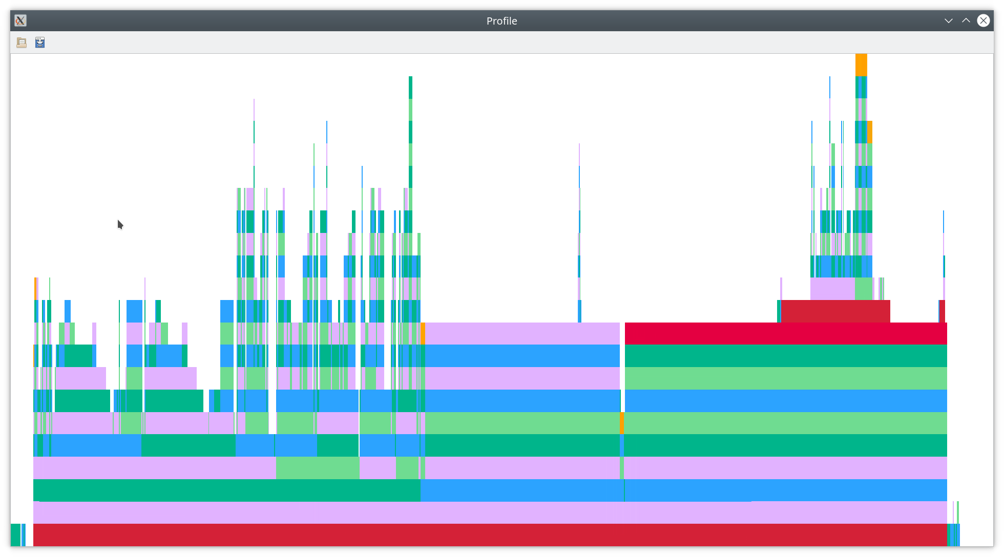
You should see something like the following flamegraph.

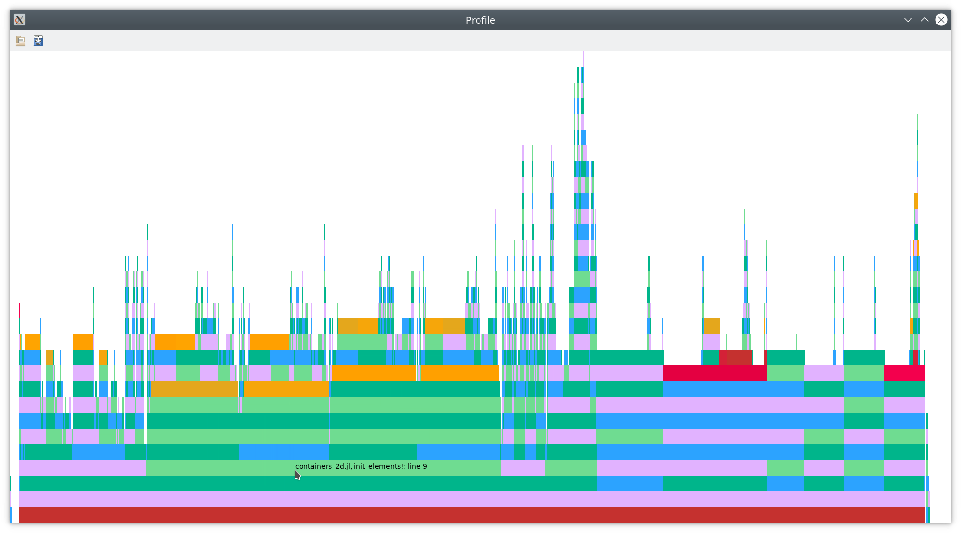
As you can see there, most of the time is spend in line 9 of init_elements! (near the mouse cursor), which is reproduced below.

# Initialize data structures in element container
function init_elements!(elements, mesh::P4estMesh{2}, basis::LobattoLegendreBasis)
  @unpack node_coordinates, jacobian_matrix,
          contravariant_vectors, inverse_jacobian = elements

  calc_node_coordinates!(node_coordinates, mesh, basis.nodes)

  for element in 1:ncells(mesh)
    calc_jacobian_matrix!(jacobian_matrix, element, node_coordinates, basis)

    calc_contravariant_vectors!(contravariant_vectors, element, jacobian_matrix)

    calc_inverse_jacobian!(inverse_jacobian, element, jacobian_matrix)
  end

  return nothing
end

Line 9 is calc_jacobian_matrix!(jacobian_matrix, element, node_coordinates, basis). You can open this line in your favorite editor of choice (set via ENV["JULIA_EDITOR"], e.g. code for Visual Studio Code with the Julia extension in my setup) by right-clicking on the bar in the flamegraph.

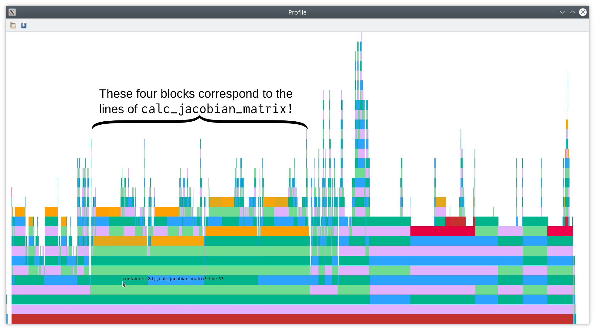
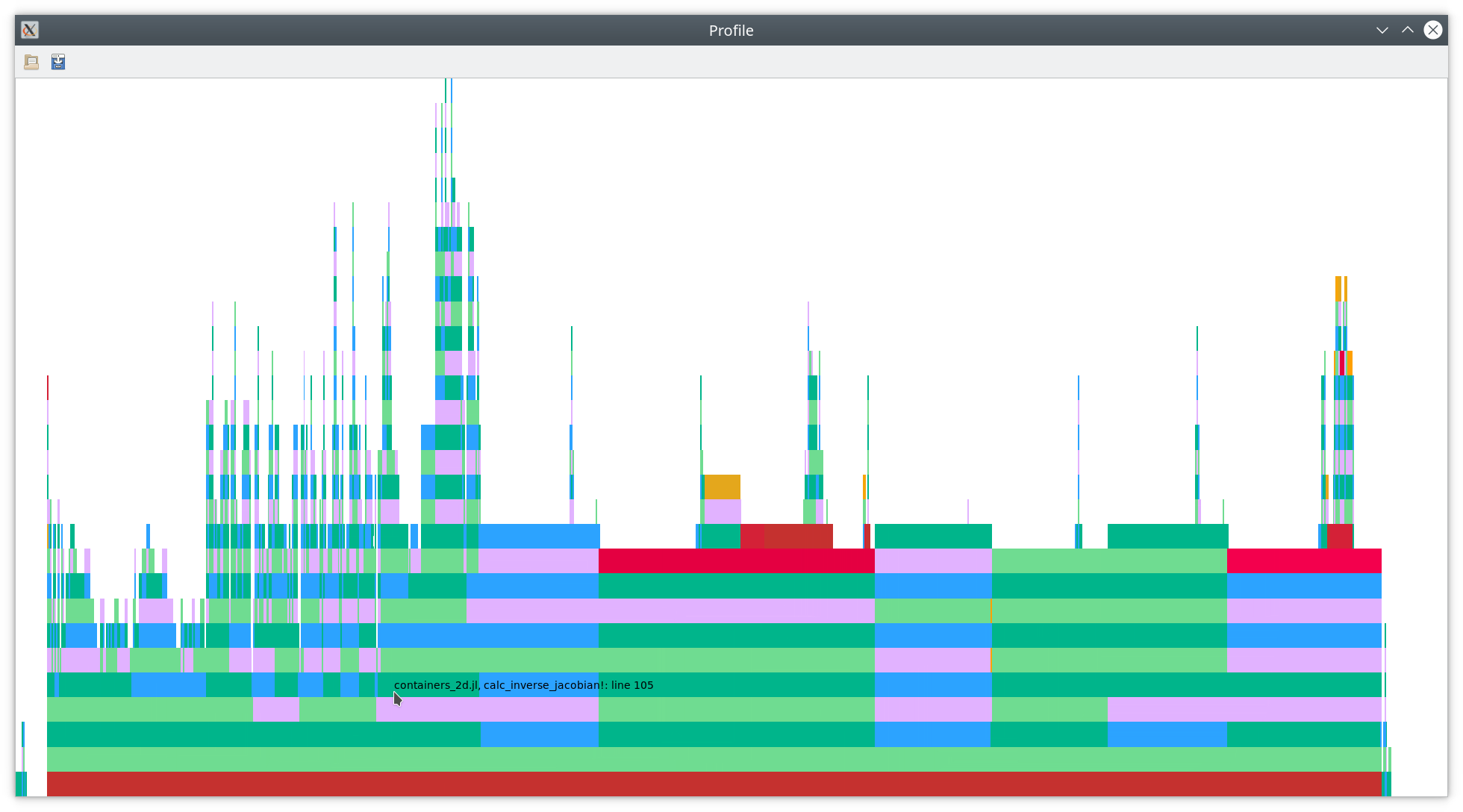
As you can see in this flamegraph, each of the four lines of

function calc_jacobian_matrix!(jacobian_matrix, element, node_coordinates::AbstractArray{<:Any, 4}, basis::LobattoLegendreBasis)
  @views mul!(jacobian_matrix[1, 1, :, :, element], basis.derivative_matrix, node_coordinates[1, :, :, element]) # x_ξ
  @views mul!(jacobian_matrix[2, 1, :, :, element], basis.derivative_matrix, node_coordinates[2, :, :, element]) # y_ξ
  @views mul!(jacobian_matrix[1, 2, :, :, element], node_coordinates[1, :, :, element], basis.derivative_matrix') # x_η
  @views mul!(jacobian_matrix[2, 2, :, :, element], node_coordinates[2, :, :, element], basis.derivative_matrix') # y_η

  return jacobian_matrix
end

takes quite some time. By climbing up the call chain, it becomes obvious that these calls to mul! end up in some generic linear algebra code of Julia (because of the views) that doesn’t really seem to be optimized a lot. We might improve the performance by reformulating this such that BLAS libraries can used. However, the sizes of the matrices are relatively small and OpenBLAS (shipped with Julia) is not really very efficient for such small matrices. We could try to swap OpenBLAS and use Intel MKL or something similar, but we can also do much better and use pure Julia code: It’s time for LoopVectorization.jl.

Before we optimize this part, let’s get some baseline values again.

julia> @benchmark Trixi.calc_jacobian_matrix!(
           $(semi.cache.elements.jacobian_matrix),
           $(1),
           $(semi.cache.elements.node_coordinates),
           $(solver.basis))
samples: 10000; evals/sample: 164; memory estimate: 896 bytes; allocs estimate: 16
ns

 (700.0   - 4000.0 ]  ██████████████████████████████ 9983
 (4000.0  - 7400.0 ]   0
 (7400.0  - 10800.0]   0
 (10800.0 - 14200.0]   0
 (14200.0 - 17600.0]   0
 (17600.0 - 21000.0]   0
 (21000.0 - 24400.0]   0
 (24400.0 - 27800.0]   0
 (27800.0 - 31200.0]   0
 (31200.0 - 34600.0]   0
 (34600.0 - 38000.0]   0
 (38000.0 - 41400.0]   0
 (41400.0 - 44800.0]   0
 (44800.0 - 48200.0]  ▏2
 (48200.0 - 51600.0]  ▏15

                  Counts

min: 650.817 ns (0.00% GC); mean: 762.658 ns (10.76% GC); median: 662.390 ns (0.00% GC); max: 51.557 μs (98.45% GC).

Let’s re-write the matrix multiplications using explicit loops and performance annotations from LoopVectorization.jl.

# Calculate Jacobian matrix of the mapping from the reference element to the element in the physical domain
function calc_jacobian_matrix!(jacobian_matrix, element, node_coordinates::AbstractArray{<:Any, 4}, basis::LobattoLegendreBasis)
  @unpack derivative_matrix = basis

  # The code below is equivalent to the following matrix multiplications, which
  # seem to end up calling generic linear algebra code from Julia. Thus, the
  # optimized code below using `@turbo` is much faster.
  # @views mul!(jacobian_matrix[1, 1, :, :, element], derivative_matrix, node_coordinates[1, :, :, element]) # x_ξ
  # @views mul!(jacobian_matrix[2, 1, :, :, element], derivative_matrix, node_coordinates[2, :, :, element]) # y_ξ
  # @views mul!(jacobian_matrix[1, 2, :, :, element], node_coordinates[1, :, :, element], derivative_matrix') # x_η
  # @views mul!(jacobian_matrix[2, 2, :, :, element], node_coordinates[2, :, :, element], derivative_matrix') # y_η

  # x_ξ, y_ξ
  @turbo for xy in indices((jacobian_matrix, node_coordinates), (1, 1))
    for j in indices((jacobian_matrix, node_coordinates), (4, 3)), i in indices((jacobian_matrix, derivative_matrix), (3, 1))
      res = zero(eltype(jacobian_matrix))
      for ii in indices((node_coordinates, derivative_matrix), (2, 2))
        res += derivative_matrix[i, ii] * node_coordinates[xy, ii, j, element]
      end
      jacobian_matrix[xy, 1, i, j, element] = res
    end
  end

  # x_η, y_η
  @turbo for xy in indices((jacobian_matrix, node_coordinates), (1, 1))
    for j in indices((jacobian_matrix, derivative_matrix), (4, 1)), i in indices((jacobian_matrix, node_coordinates), (3, 2))
      res = zero(eltype(jacobian_matrix))
      for jj in indices((node_coordinates, derivative_matrix), (3, 2))
        res += derivative_matrix[j, jj] * node_coordinates[xy, i, jj, element]
      end
      jacobian_matrix[xy, 2, i, j, element] = res
    end
  end

  return jacobian_matrix
end

On top of writing out the loops explicitly, we used two techniques to get full speed.

• @turbo from LoopVectorization.jl transforms the loops and tries to generate efficient compiled code using SIMD instructions.
• indices((jacobian_matrix, node_coordinates), (1, 1)) tells LoopVectorization.jl that the sizes of the first dimensions of jacobian_matrix and node_coordinates are the same and that we iterate over the full first dimension. That’s more information than available from something like axes(jacobian_matrix, 1), so it allows LoopVectorization.jl to take advantage of it and generate better code.

Let’s have a look at the resulting performance.

julia> @benchmark Trixi.calc_jacobian_matrix!(
           $(semi.cache.elements.jacobian_matrix),
           $(1),
           $(semi.cache.elements.node_coordinates),
           $(solver.basis))
samples: 10000; evals/sample: 987; memory estimate: 0 bytes; allocs estimate: 0
ns

 (49.9  - 53.6 ]  ██████████████████████████████ 9800
 (53.6  - 57.4 ]  ▏10
 (57.4  - 61.1 ]  ▏2
 (61.1  - 64.9 ]  ▎51
 (64.9  - 68.6 ]  ▎47
 (68.6  - 72.3 ]  ▏4
 (72.3  - 76.1 ]  ▏1
 (76.1  - 79.8 ]  ▎44
 (79.8  - 83.6 ]  ▏16
 (83.6  - 87.3 ]  ▏4
 (87.3  - 91.1 ]  ▏3
 (91.1  - 94.8 ]  ▏3
 (94.8  - 98.6 ]  ▏4
 (98.6  - 102.3]  ▏1
 (102.3 - 115.8]  ▏10

                  Counts

min: 49.875 ns (0.00% GC); mean: 50.854 ns (0.00% GC); median: 50.369 ns (0.00% GC); max: 115.848 ns (0.00% GC).

That’s an impressive speed-up from ca. 700 nanoseconds to ca. 50 nanoseconds per element! Since we optimized a part that took a relatively large amount of the total run time, we also get a decent speed-up of reinitialize_containers!.

julia> @benchmark Trixi.reinitialize_containers!($mesh, $equations, $solver, $(semi.cache))
samples: 6735; evals/sample: 1; memory estimate: 418.16 KiB; allocs estimate: 4953
ns

 (690000.0 - 1.22e6]  ██████████████████████████████ 6702
 (1.22e6   - 1.75e6]  ▏1
 (1.75e6   - 2.28e6]   0
 (2.28e6   - 2.81e6]   0
 (2.81e6   - 3.34e6]   0
 (3.34e6   - 3.87e6]   0
 (3.87e6   - 4.4e6 ]   0
 (4.4e6    - 4.94e6]   0
 (4.94e6   - 5.47e6]   0
 (5.47e6   - 6.0e6 ]   0
 (6.0e6    - 6.53e6]   0
 (6.53e6   - 7.06e6]   0
 (7.06e6   - 7.59e6]  ▏6
 (7.59e6   - 8.12e6]  ▏26

                  Counts

min: 688.565 μs (0.00% GC); mean: 739.861 μs (4.46% GC); median: 694.888 μs (0.00% GC); max: 8.120 ms (90.25% GC).

The runtime of this part is reduced by ca. 25%.

Step 2: Attack the next major performance impact

Let’s repeat the profiling to find our next goal for further optimizations.

julia> @profview doit(mesh, equations, solver, semi.cache, 10^4)

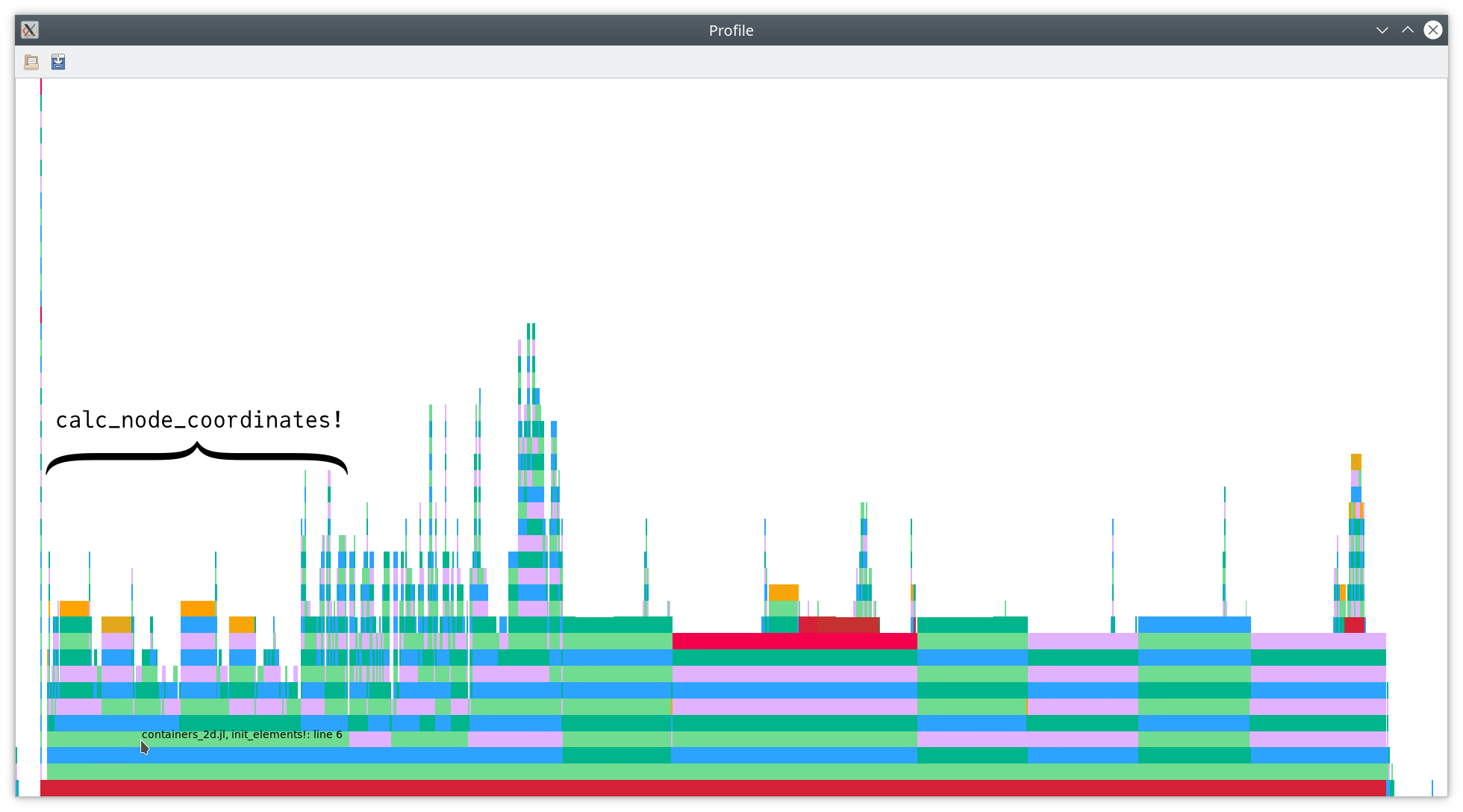
As you can see above, the next big block is calc_node_coordinates!(node_coordinates, mesh, basis.nodes). Let’s get some baseline values.

julia> @benchmark Trixi.calc_node_coordinates!(
           $(semi.cache.elements.node_coordinates),
           $(mesh),
           $(solver.basis.nodes))
samples: 10000; evals/sample: 1; memory estimate: 284.05 KiB; allocs estimate: 1795
ns

 (130000.0 - 560000.0]  ██████████████████████████████▏9967
 (560000.0 - 1.0e6   ]   0
 (1.0e6    - 1.44e6  ]   0
 (1.44e6   - 1.88e6  ]   0
 (1.88e6   - 2.32e6  ]   0
 (2.32e6   - 2.75e6  ]   0
 (2.75e6   - 3.19e6  ]   0
 (3.19e6   - 3.63e6  ]   0
 (3.63e6   - 4.07e6  ]   0
 (4.07e6   - 4.51e6  ]   0
 (4.51e6   - 4.94e6  ]   0
 (4.94e6   - 5.38e6  ]   0
 (5.38e6   - 5.82e6  ]   0
 (5.82e6   - 6.26e6  ]  ▏23
 (6.26e6   - 8.23e6  ]  ▏10

                  Counts

min: 126.054 μs (0.00% GC); mean: 173.450 μs (11.67% GC); median: 130.181 μs (0.00% GC); max: 8.228 ms (97.68% GC).

To improve the performance, let’s dig deeper in the flamegraph.

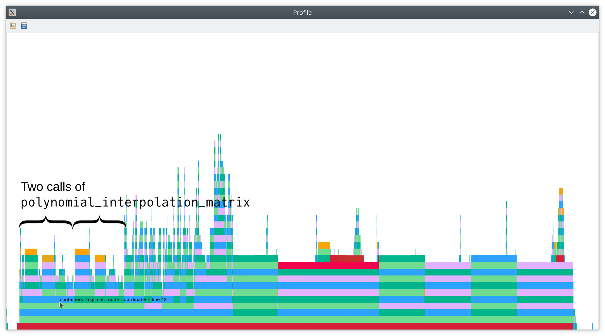
Most of the time here is spent in the two lines

matrix1 = polynomial_interpolation_matrix(mesh.nodes, nodes_out_x)
matrix2 = polynomial_interpolation_matrix(mesh.nodes, nodes_out_y)

Let’s see what’s going on:

# Calculate and interpolation matrix (Vandermonde matrix) between two given sets of nodes
function polynomial_interpolation_matrix(nodes_in, nodes_out)
  n_nodes_in = length(nodes_in)
  n_nodes_out = length(nodes_out)
  wbary_in = barycentric_weights(nodes_in)
  vdm = zeros(n_nodes_out, n_nodes_in)

  for k in 1:n_nodes_out
    match = false
    for j in 1:n_nodes_in
      if isapprox(nodes_out[k], nodes_in[j], rtol=eps())
        match = true
        vdm[k, j] = 1
      end
    end

    if match == false
      s = 0.0
      for j in 1:n_nodes_in
        t = wbary_in[j] / (nodes_out[k] - nodes_in[j])
        vdm[k, j] = t
        s += t
      end
      for j in 1:n_nodes_in
        vdm[k, j] = vdm[k, j] / s
      end
    end
  end

  return vdm
end

Clearly, there will be a lot of repeated allocations if we use this method as it is. To be fair, this method was written in the very early days of Trixi. Back in these days, it was only used at the very beginning when initializing the DGSEM solver and necessary interpolation matrices. Hence, it was never critical for performance at that time. Now, it has become a bottleneck and needs to be improved.

Let’s implement the core logic without allocations in another function.

# Calculate and interpolation matrix (Vandermonde matrix) between two given sets of nodes
function polynomial_interpolation_matrix(nodes_in, nodes_out,
                                         baryweights_in=barycentric_weights(nodes_in))
  n_nodes_in = length(nodes_in)
  n_nodes_out = length(nodes_out)
  vandermonde = Matrix{promote_type(eltype(nodes_in), eltype(nodes_out))}(undef,
                  n_nodes_out, n_nodes_in)
  polynomial_interpolation_matrix!(vandermonde, nodes_in, nodes_out, baryweights_in)

  return vandermonde
end

function polynomial_interpolation_matrix!(vandermonde,
                                          nodes_in, nodes_out,
                                          baryweights_in)
  fill!(vandermonde, zero(eltype(vandermonde)))

  for k in eachindex(nodes_out)
    match = false
    for j in eachindex(nodes_in)
      if isapprox(nodes_out[k], nodes_in[j])
        match = true
        vandermonde[k, j] = 1
      end
    end

    if match == false
      s = zero(eltype(vandermonde))
      for j in eachindex(nodes_in)
        t = baryweights_in[j] / (nodes_out[k] - nodes_in[j])
        vandermonde[k, j] = t
        s += t
      end
      for j in eachindex(nodes_in)
        vandermonde[k, j] = vandermonde[k, j] / s
      end
    end
  end

  return vandermonde
end

This approach is good practice in Julia: Write efficient in-place versions without allocations and easy-to-use allocating versions additionally.

If we move the allocations

baryweights_in = barycentric_weights(mesh.nodes)
matrix1 = Matrix{real(mesh)}(undef, length(nodes), length(mesh.nodes))
matrix2 = similar(matrix1)

to calc_node_coordinates! and use the in-place versions

polynomial_interpolation_matrix!(matrix1, mesh.nodes, nodes_out_x, baryweights_in)
polynomial_interpolation_matrix!(matrix2, mesh.nodes, nodes_out_y, baryweights_in)

in the loop, we get the following results.

julia> @benchmark Trixi.calc_node_coordinates!(
           $(semi.cache.elements.node_coordinates),
           $(mesh),
           $(solver.basis.nodes))
samples: 10000; evals/sample: 1; memory estimate: 4.56 KiB; allocs estimate: 6
ns

 (101400.0 - 106600.0]  ██████████████████████████████ 9562
 (106600.0 - 111800.0]  ▍82
 (111800.0 - 117000.0]  ▍81
 (117000.0 - 122200.0]  ▏36
 (122200.0 - 127400.0]  ▏4
 (127400.0 - 132600.0]  ▌135
 (132600.0 - 137800.0]  ▏20
 (137800.0 - 143000.0]  ▏3
 (143000.0 - 148200.0]  ▏23
 (148200.0 - 153400.0]  ▏10
 (153400.0 - 158600.0]  ▏13
 (158600.0 - 163800.0]  ▏15
 (163800.0 - 169000.0]  ▏2
 (169000.0 - 174200.0]  ▏4
 (174200.0 - 346600.0]  ▏10

                  Counts

min: 101.423 μs (0.00% GC); mean: 103.452 μs (0.00% GC); median: 102.124 μs (0.00% GC); max: 346.622 μs (0.00% GC).

julia> @benchmark Trixi.reinitialize_containers!($mesh, $equations, $solver, $(semi.cache))
samples: 7159; evals/sample: 1; memory estimate: 138.67 KiB; allocs estimate: 3164
ns

 (700000.0 - 1.4e6 ]  ██████████████████████████████7148
 (1.4e6    - 2.2e6 ]   0
 (2.2e6    - 3.0e6 ]   0
 (3.0e6    - 3.8e6 ]   0
 (3.8e6    - 4.6e6 ]   0
 (4.6e6    - 5.4e6 ]   0
 (5.4e6    - 6.2e6 ]   0
 (6.2e6    - 6.9e6 ]   0
 (6.9e6    - 7.7e6 ]   0
 (7.7e6    - 8.5e6 ]   0
 (8.5e6    - 9.3e6 ]   0
 (9.3e6    - 1.01e7]   0
 (1.01e7   - 1.09e7]   0
 (1.09e7   - 1.16e7]  ▏11

                  Counts

min: 664.983 μs (0.00% GC); mean: 695.805 μs (2.38% GC); median: 669.974 μs (0.00% GC); max: 11.649 ms (93.42% GC).

Thus, pre-allocating some storage reduced the runtime of calc_node_coordinates! by ca. 25%, gaining ca. 5% better performance of reinitialize_containers!.

Step 3: Another step towards improved performance

There is still some room for further improvements. Looking at the new flamegraph below, we see that the next reasonable target of our optimizations is calc_inverse_jacobian!(inverse_jacobian, element, jacobian_matrix) in init_elements!, which is reproduced below for convenience.

# Calculate inverse Jacobian (determinant of Jacobian matrix of the mapping) in each node
function calc_inverse_jacobian!(inverse_jacobian::AbstractArray{<:Any,3}, element, jacobian_matrix)
  @. @views inverse_jacobian[:, :, element] = inv(jacobian_matrix[1, 1, :, :, element] * jacobian_matrix[2, 2, :, :, element] -
                                                  jacobian_matrix[1, 2, :, :, element] * jacobian_matrix[2, 1, :, :, element])

  return inverse_jacobian
end

The baseline timing is

julia> @benchmark Trixi.calc_inverse_jacobian!(
           $(semi.cache.elements.inverse_jacobian),
           $(1),
           $(semi.cache.elements.jacobian_matrix))
samples: 10000; evals/sample: 935; memory estimate: 0 bytes; allocs estimate: 0
ns

 (106.0 - 119.0]  ██████████████████████████████ 8277
 (119.0 - 131.0]  █▋448
 (131.0 - 143.0]  █▏306
 (143.0 - 155.0]  █248
 (155.0 - 168.0]  ▊200
 (168.0 - 180.0]  ▊184
 (180.0 - 192.0]  ▌121
 (192.0 - 204.0]  ▍90
 (204.0 - 217.0]  ▏31
 (217.0 - 229.0]  ▏23
 (229.0 - 241.0]  ▏24
 (241.0 - 253.0]  ▏16
 (253.0 - 266.0]  ▏14
 (266.0 - 278.0]  ▏8
 (278.0 - 321.0]  ▏10

                  Counts

min: 106.279 ns (0.00% GC); mean: 117.476 ns (0.00% GC); median: 109.401 ns (0.00% GC); max: 321.129 ns (0.00% GC).

Throwing in some performance optimizations using LoopVectorization.jl, we end up with the code

# Calculate inverse Jacobian (determinant of Jacobian matrix of the mapping) in each node
function calc_inverse_jacobian!(inverse_jacobian::AbstractArray{<:Any,3}, element, jacobian_matrix)
  # The code below is equivalent to the following high-level code but much faster.
  # @. @views inverse_jacobian[:, :, element] = inv(jacobian_matrix[1, 1, :, :, element] * jacobian_matrix[2, 2, :, :, element] -
  #                                                 jacobian_matrix[1, 2, :, :, element] * jacobian_matrix[2, 1, :, :, element])

  @turbo for j in indices((inverse_jacobian, jacobian_matrix), (2, 4)),
             i in indices((inverse_jacobian, jacobian_matrix), (1, 3))
    inverse_jacobian[i, j, element] = inv(jacobian_matrix[1, 1, i, j, element] * jacobian_matrix[2, 2, i, j, element] -
                                          jacobian_matrix[1, 2, i, j, element] * jacobian_matrix[2, 1, i, j, element])
  end

  return inverse_jacobian
end

and the benchmark results

julia> @benchmark Trixi.calc_inverse_jacobian!(
           $(semi.cache.elements.inverse_jacobian),
           $(1),
           $(semi.cache.elements.jacobian_matrix))
samples: 10000; evals/sample: 999; memory estimate: 0 bytes; allocs estimate: 0
ns

 (12.7 - 13.8]  ██████████████████████████████ 9905
 (13.8 - 15.0]  ▏25
 (15.0 - 16.1]  ▏11
 (16.1 - 17.2]   0
 (17.2 - 18.3]   0
 (18.3 - 19.4]   0
 (19.4 - 20.5]  ▏1
 (20.5 - 21.6]   0
 (21.6 - 22.7]   0
 (22.7 - 23.8]   0
 (23.8 - 24.9]   0
 (24.9 - 26.0]  ▏19
 (26.0 - 27.1]  ▏10
 (27.1 - 28.2]  ▏19
 (28.2 - 38.7]  ▏10

                  Counts

min: 12.740 ns (0.00% GC); mean: 12.847 ns (0.00% GC); median: 12.754 ns (0.00% GC); max: 38.741 ns (0.00% GC).

julia> @benchmark Trixi.reinitialize_containers!($mesh, $equations, $solver, $(semi.cache))
samples: 7647; evals/sample: 1; memory estimate: 138.67 KiB; allocs estimate: 3164
ns

 (600000.0 - 1.4e6 ]  ██████████████████████████████7635
 (1.4e6    - 2.3e6 ]   0
 (2.3e6    - 3.1e6 ]   0
 (3.1e6    - 3.9e6 ]   0
 (3.9e6    - 4.7e6 ]   0
 (4.7e6    - 5.5e6 ]   0
 (5.5e6    - 6.3e6 ]   0
 (6.3e6    - 7.1e6 ]   0
 (7.1e6    - 8.0e6 ]   0
 (8.0e6    - 8.8e6 ]   0
 (8.8e6    - 9.6e6 ]   0
 (9.6e6    - 1.04e7]   0
 (1.04e7   - 1.12e7]   0
 (1.12e7   - 1.2e7 ]  ▏12

                  Counts

min: 621.222 μs (0.00% GC); mean: 651.399 μs (2.66% GC); median: 626.502 μs (0.00% GC); max: 12.040 ms (93.98% GC).

The gain from these single performance improvements becomes smaller since our targets contribute less to the overall runtime. Here, we gained ca. 7 percent improvement for reinitialize_containers!.

By the way, I discovered a bug in LoopVectorization.jl while performing a quick smoke test after this change. Chris Elrod, the author of LoopVectorization.jl fixed this very quickly after reporting it - great support, as always!

Step 4: Iterating further

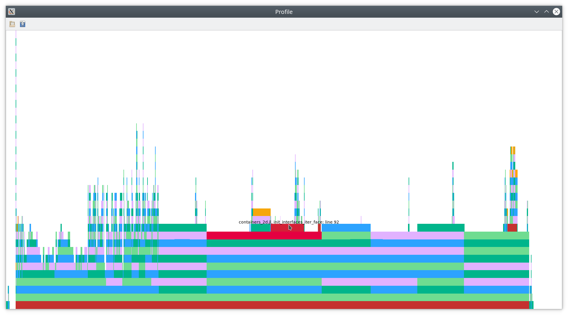
Next, we will dig into init_interfaces!. As you can see in the flamegraph below, there is a realtively large red part at the top, indicating type instabilities and dynamic dispatch.

Let’s get some baseline numbers.

julia> @benchmark Trixi.init_interfaces!($(semi.cache.interfaces), $mesh)
samples: 10000; evals/sample: 1; memory estimate: 108.08 KiB; allocs estimate: 2789
ns

 (100000.0 - 800000.0]  ██████████████████████████████▏9988
 (800000.0 - 1.5e6   ]   0
 (1.5e6    - 2.2e6   ]   0
 (2.2e6    - 2.9e6   ]   0
 (2.9e6    - 3.6e6   ]   0
 (3.6e6    - 4.3e6   ]   0
 (4.3e6    - 5.0e6   ]   0
 (5.0e6    - 5.7e6   ]   0
 (5.7e6    - 6.4e6   ]   0
 (6.4e6    - 7.1e6   ]   0
 (7.1e6    - 7.8e6   ]   0
 (7.8e6    - 8.5e6   ]   0
 (8.5e6    - 9.2e6   ]   0
 (9.2e6    - 9.9e6   ]   0
 (9.9e6    - 1.06e7  ]  ▏12

                  Counts

min: 119.396 μs (0.00% GC); mean: 135.710 μs (8.85% GC); median: 121.333 μs (0.00% GC); max: 10.552 ms (98.60% GC).

The code yielding the red parts in the flamegraph that we will target now is

# Iterate over all interfaces and extract inner interface data to interface container
# This function will be passed to p4est in init_interfaces! below
function init_interfaces_iter_face(info, user_data)
  if info.sides.elem_count != 2
    # Not an inner interface
    return nothing
  end

  sides = (load_sc_array(p4est_iter_face_side_t, info.sides, 1),
           load_sc_array(p4est_iter_face_side_t, info.sides, 2))

  if sides[1].is_hanging == true || sides[2].is_hanging == true
    # Mortar, no normal interface
    return nothing
  end

  # Unpack user_data = [interfaces, interface_id, mesh] and increment interface_id
  ptr = Ptr{Any}(user_data)
  data_array = unsafe_wrap(Array, ptr, 3)
  interfaces = data_array[1]
  interface_id = data_array[2]
  data_array[2] = interface_id + 1
  mesh = data_array[3]

  # Function barrier because the unpacked user_data above is type-unstable
  init_interfaces_iter_face_inner(info, sides, interfaces, interface_id, mesh)
end

This code is much more difficult to optimize since we’re dealing not only with Julia code but interface the p4est library written in C. Thus, we need to live with some restrictions and can’t use multiple dispatch for user_data. Instead, we just get some Ptr{Nothing} and that’s it.

One minor modification we can make is to avoid calling unsafe_wrap(Array, ...), since this comes with some overhead, both when wrapping the array and when loading data from it (type instabilities occur since data_array isa Vector{Any}). Since we’re only loading non-homogeneous items a few times from ptr, we can use unsafe_load instead.

# Iterate over all interfaces and extract inner interface data to interface container
# This function will be passed to p4est in init_interfaces! below
function init_interfaces_iter_face(info, user_data)
  if info.sides.elem_count != 2
    # Not an inner interface
    return nothing
  end

  sides = (load_sc_array(p4est_iter_face_side_t, info.sides, 1),
           load_sc_array(p4est_iter_face_side_t, info.sides, 2))

  if sides[1].is_hanging == true || sides[2].is_hanging == true
    # Mortar, no normal interface
    return nothing
  end

  # Unpack user_data = [interfaces, interface_id, mesh] and increment interface_id
  ptr = Ptr{Any}(user_data)
  interfaces   = unsafe_load(ptr, 1)
  interface_id = unsafe_load(ptr, 2)
  mesh         = unsafe_load(ptr, 3)
  unsafe_store!(ptr, interface_id + 1, 2)

  # Function barrier because the unpacked user_data above is type-unstable
  init_interfaces_iter_face_inner(info, sides, interfaces, interface_id, mesh)
end

The performance of this part improved by ca. 10%, yielding a speed-up of reinitialize_containers! of ca. 4%. Of course, I also searched for unsafe_wrap in the same file and replaced similar parts in init_mortars_iter_face and init_boundaries_iter_face (which are not shown in this post).

julia> @benchmark Trixi.init_interfaces!($(semi.cache.interfaces), $mesh)
samples: 10000; evals/sample: 1; memory estimate: 43.70 KiB; allocs estimate: 1965
ns

 (105000.0 - 118000.0]  ██████████████████████████████ 7980
 (118000.0 - 132000.0]  ██▊712
 (132000.0 - 145000.0]  █262
 (145000.0 - 158000.0]  ▉201
 (158000.0 - 172000.0]  ▋150
 (172000.0 - 185000.0]  ▋136
 (185000.0 - 199000.0]  ▊180
 (199000.0 - 212000.0]  ▋163
 (212000.0 - 225000.0]  ▍91
 (225000.0 - 239000.0]  ▎48
 (239000.0 - 252000.0]  ▏30
 (252000.0 - 266000.0]  ▏20
 (266000.0 - 279000.0]  ▏11
 (279000.0 - 292000.0]  ▏6
 (292000.0 - 8.416e6 ]  ▏10

                  Counts

min: 104.825 μs (0.00% GC); mean: 123.543 μs (3.10% GC); median: 110.587 μs (0.00% GC); max: 8.416 ms (97.23% GC).

julia> @benchmark Trixi.reinitialize_containers!($mesh, $equations, $solver, $(semi.cache))
samples: 7976; evals/sample: 1; memory estimate: 74.30 KiB; allocs estimate: 2340
ns

 (603000.0 - 633000.0]  ██████████████████████████████▏6758
 (633000.0 - 662000.0]  ████879
 (662000.0 - 691000.0]  ▉197
 (691000.0 - 721000.0]  ▎39
 (721000.0 - 750000.0]  ▏24
 (750000.0 - 779000.0]  ▏22
 (779000.0 - 808000.0]  ▏25
 (808000.0 - 838000.0]  ▏8
 (838000.0 - 867000.0]  ▏9
 (867000.0 - 896000.0]  ▏3
 (896000.0 - 925000.0]  ▏2
 (925000.0 - 955000.0]   0
 (955000.0 - 984000.0]  ▏2
 (984000.0 - 1.1112e7]  ▏8

                  Counts

min: 603.419 μs (0.00% GC); mean: 624.644 μs (1.42% GC); median: 607.376 μs (0.00% GC); max: 11.112 ms (93.67% GC).

Since there are still type instabilities and allocations in init_interfaces!, there should still be room for further improvements. However, it looks like these would require further restructuring and more complicated techniques. We will revisit this part later.

Step 5: Another look at init_elements!

Let’s have another look at init_elements!, the most expensive part we’re trying to improve.

# Initialize data structures in element container
function init_elements!(elements, mesh::P4estMesh{2}, basis::LobattoLegendreBasis)
  @unpack node_coordinates, jacobian_matrix,
          contravariant_vectors, inverse_jacobian = elements

  calc_node_coordinates!(node_coordinates, mesh, basis.nodes)

  for element in 1:ncells(mesh)
    calc_jacobian_matrix!(jacobian_matrix, element, node_coordinates, basis)

    calc_contravariant_vectors!(contravariant_vectors, element, jacobian_matrix)

    calc_inverse_jacobian!(inverse_jacobian, element, jacobian_matrix)
  end

  return nothing
end

We have already optimized calc_jacobian_matrix! and calc_inverse_jacobian!. Next, we improve the performance of calc_contravariant_vectors!. Using the same approach as before, we rewrite broadcasting operations into loops using @turbo from LoopVectorization.jl, ending up with

# Calculate contravarant vectors, multiplied by the Jacobian determinant J of the transformation mapping.
# Those are called Ja^i in Kopriva's blue book.
function calc_contravariant_vectors!(contravariant_vectors::AbstractArray{<:Any,5}, element, jacobian_matrix)
  # The code below is equivalent to the following using broadcasting but much faster.
  # # First contravariant vector Ja^1
  # @. @views contravariant_vectors[1, 1, :, :, element] =  jacobian_matrix[2, 2, :, :, element]
  # @. @views contravariant_vectors[2, 1, :, :, element] = -jacobian_matrix[1, 2, :, :, element]
  # # Second contravariant vector Ja^2
  # @. @views contravariant_vectors[1, 2, :, :, element] = -jacobian_matrix[2, 1, :, :, element]
  # @. @views contravariant_vectors[2, 2, :, :, element] =  jacobian_matrix[1, 1, :, :, element]

  @turbo for j in indices((contravariant_vectors, jacobian_matrix), (4, 4)),
             i in indices((contravariant_vectors, jacobian_matrix), (3, 3))
    # First contravariant vector Ja^1
    contravariant_vectors[1, 1, i, j, element] =  jacobian_matrix[2, 2, i, j, element]
    contravariant_vectors[2, 1, i, j, element] = -jacobian_matrix[1, 2, i, j, element]

    # Second contravariant vector Ja^2
    contravariant_vectors[1, 2, i, j, element] = -jacobian_matrix[2, 1, i, j, element]
    contravariant_vectors[2, 2, i, j, element] =  jacobian_matrix[1, 1, i, j, element]
  end

  return contravariant_vectors
end

Again, we got a speed-up of ca. 5% for reinitialize_containers!.

julia> @benchmark Trixi.reinitialize_containers!($mesh, $equations, $solver, $(semi.cache))
samples: 8406; evals/sample: 1; memory estimate: 66.05 KiB; allocs estimate: 2244
ns

 (575000.0 - 600000.0]  ██████████████████████████████ 7342
 (600000.0 - 624000.0]  ███▎768
 (624000.0 - 649000.0]  ▉188
 (649000.0 - 673000.0]  ▎42
 (673000.0 - 698000.0]  ▏23
 (698000.0 - 723000.0]  ▏9
 (723000.0 - 747000.0]  ▏5
 (747000.0 - 772000.0]  ▏6
 (772000.0 - 797000.0]  ▏4
 (797000.0 - 821000.0]  ▏2
 (821000.0 - 846000.0]  ▏1
 (846000.0 - 871000.0]  ▏4
 (871000.0 - 895000.0]  ▏2
 (895000.0 - 920000.0]  ▏1
 (920000.0 - 1.0221e7]  ▏9

                  Counts

min: 574.922 μs (0.00% GC); mean: 592.397 μs (1.13% GC); median: 579.274 μs (0.00% GC); max: 10.221 ms (92.91% GC).

By the way, this optimization discovered another bug in LoopVectorization.jl. As always, Chris Elrod was very helpful and fixed the bug quite fast.

Step 6: Passing more information at compile time

Let’s see what we have achieved so far by looking at the current flamegraph.

julia> @profview doit(mesh, equations, solver, semi.cache, 10^4)

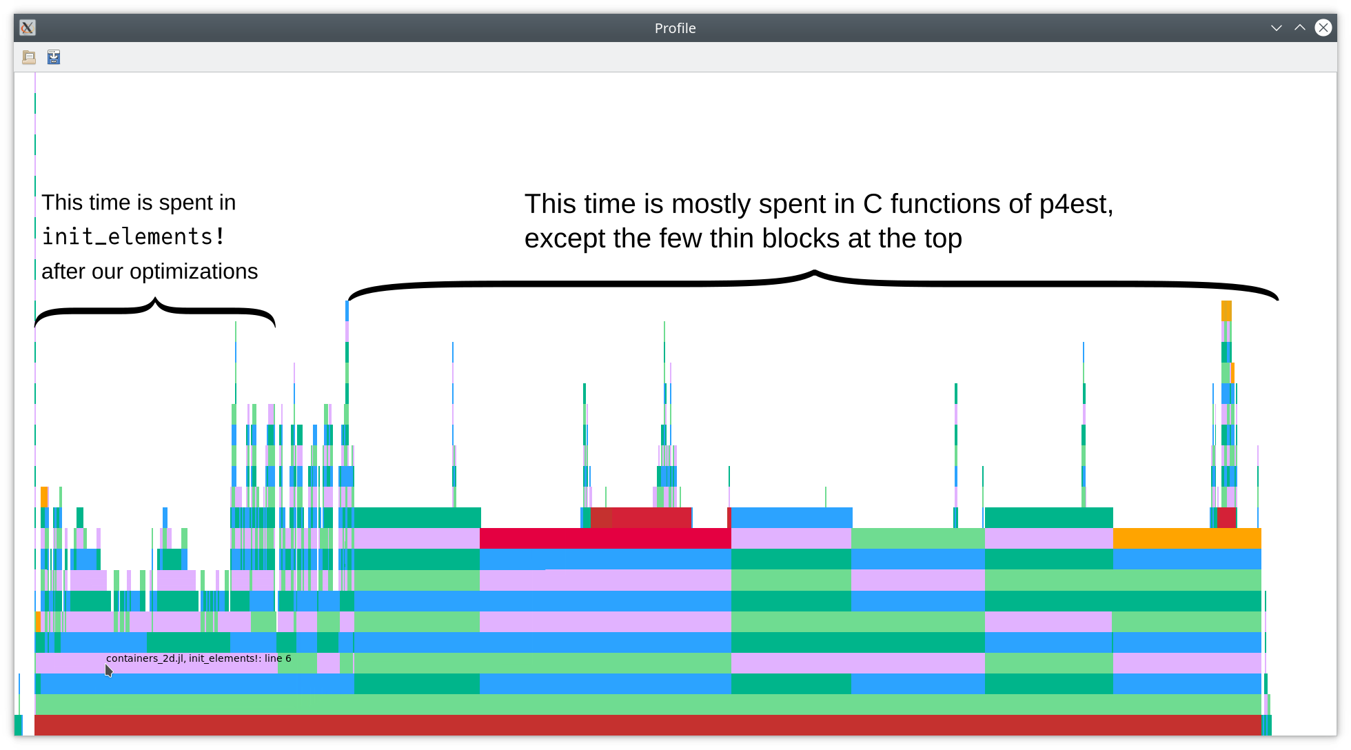
This is already much better than what we had at the beginning: Ca. 70% of the total time is spent inside p4est functions (p4est_iterate). The only one of these calls where Julia code takes a significant amount of the time is init_interfaces_iter_face, which is type-unstable as discussed above.

Nevertheless, there is still more room for improvements of the remaining Julia code. While LoopVectorization.jl and its code generation capabilities are great, they can only work with information available to them and need to make some reasonable heuristics. In particular, they do not know the small sizes of some arrays such as the polynomial interpolation matrices used in calc_node_coordinates!. Let’s change that!

First, we need to make sure that the important size information is available at compile time. Thus, we change the definition of the P4estMesh from

mutable struct P4estMesh{NDIMS, RealT<:Real, NDIMSP2} <: AbstractMesh{NDIMS}
  p4est                 ::Ptr{p4est_t}
  # Coordinates at the nodes specified by the tensor product of `nodes` (NDIMS times).
  # This specifies the geometry interpolation for each tree.
  tree_node_coordinates ::Array{RealT, NDIMSP2} # [dimension, i, j, k, tree]
  nodes                 ::Vector{RealT}
  boundary_names        ::Array{Symbol, 2}      # [face direction, tree]
  current_filename      ::String
  unsaved_changes       ::Bool
end

to

mutable struct P4estMesh{NDIMS, RealT<:Real, NDIMSP2, Nodes<:AbstractVector{RealT}} <: AbstractMesh{NDIMS}
  p4est                 ::Ptr{p4est_t}
  # Coordinates at the nodes specified by the tensor product of `nodes` (NDIMS times).
  # This specifies the geometry interpolation for each tree.
  tree_node_coordinates ::Array{RealT, NDIMSP2} # [dimension, i, j, k, tree]
  nodes                 ::Nodes
  boundary_names        ::Array{Symbol, 2}      # [face direction, tree]
  current_filename      ::String
  unsaved_changes       ::Bool
end

This allows us to use more general types for the nodes. In particular, we can use an SVector from StaticArrays.jl. This SVector (short form of “static vector”) carries some static size information available at compile time. After changing this type definition, we also need to adapt the constructors (function P4estMesh(...)) accordingly.

Having done that, let’s make use of the additional static size information inside calc_node_coordinates!.

# Interpolate tree_node_coordinates to each quadrant
function calc_node_coordinates!(node_coordinates,
                                mesh::P4estMesh{2},
                                basis::LobattoLegendreBasis)
  # Hanging nodes will cause holes in the mesh if its polydeg is higher
  # than the polydeg of the solver.
  @assert length(basis.nodes) >= length(mesh.nodes) "The solver can't have a lower polydeg than the mesh"

  # We use `StrideArray`s here since these buffers are used in performance-critical
  # places and the additional information passed to the compiler makes them faster
  # than native `Array`s.
  tmp1    = StrideArray(undef, real(mesh),
                        StaticInt(2), static_length(basis.nodes), static_length(mesh.nodes))
  matrix1 = StrideArray(undef, real(mesh),
                        static_length(basis.nodes), static_length(mesh.nodes))
  matrix2 = similar(matrix1)
  baryweights_in = barycentric_weights(mesh.nodes)

  # Macros from p4est
  p4est_root_len = 1 << P4EST_MAXLEVEL
  p4est_quadrant_len(l) = 1 << (P4EST_MAXLEVEL - l)

  trees = convert_sc_array(p4est_tree_t, mesh.p4est.trees)

  for tree in eachindex(trees)
    offset = trees[tree].quadrants_offset
    quadrants = convert_sc_array(p4est_quadrant_t, trees[tree].quadrants)

    for i in eachindex(quadrants)
      element = offset + i
      quad = quadrants[i]

      quad_length = p4est_quadrant_len(quad.level) / p4est_root_len

      nodes_out_x = 2 * (quad_length * 1/2 * (basis.nodes .+ 1) .+ quad.x / p4est_root_len) .- 1
      nodes_out_y = 2 * (quad_length * 1/2 * (basis.nodes .+ 1) .+ quad.y / p4est_root_len) .- 1
      polynomial_interpolation_matrix!(matrix1, mesh.nodes, nodes_out_x, baryweights_in)
      polynomial_interpolation_matrix!(matrix2, mesh.nodes, nodes_out_y, baryweights_in)

      multiply_dimensionwise!(
        view(node_coordinates, :, :, :, element),
        matrix1, matrix2,
        view(mesh.tree_node_coordinates, :, :, :, tree),
        tmp1
      )
    end
  end

  return node_coordinates
end

The function static_length is basically the same as length from Base but returns StaticInts whenver possible. These StaticInts are singletons encoding the value in their types. Thus, the size information is available at compile time and can be used to construct StrideArrays (from StrideArrays.jl) with statically known size information. This allows LoopVectorization.jl to use more information and will generally result in better performance.

Be aware that not all other libraries can handle general array types. For example, HDF5.jl wraps the C library HDF5 and doesn’t work with SVectors. Thus, we need to change the line

file["nodes"] = mesh.nodes

in function save_mesh_file(mesh::P4estMesh, output_directory, timestep=0) to

file["nodes"] = Vector(mesh.nodes) # the mesh might use custom array types
                                   # to increase the runtime performance
                                   # but HDF5 can only handle plain arrays

We also need to restart Julia since Revise.jl cannot handle redefinitions of types. After running the initialization code again, we get the following benchmark results.

julia> @benchmark Trixi.reinitialize_containers!($mesh, $equations, $solver, $(semi.cache))
samples: 8834; evals/sample: 1; memory estimate: 65.86 KiB; allocs estimate: 2244
ns

 (547000.0 - 579000.0]  ██████████████████████████████ 8078
 (579000.0 - 610000.0]  ██▌640
 (610000.0 - 642000.0]  ▍82
 (642000.0 - 674000.0]  ▏9
 (674000.0 - 706000.0]  ▏6
 (706000.0 - 738000.0]  ▏1
 (738000.0 - 770000.0]  ▏2
 (770000.0 - 802000.0]  ▏1
 (802000.0 - 834000.0]  ▏3
 (834000.0 - 866000.0]   0
 (866000.0 - 898000.0]   0
 (898000.0 - 930000.0]  ▏1
 (930000.0 - 961000.0]   0
 (961000.0 - 993000.0]  ▏2
 (993000.0 - 9.599e6 ]  ▏9

                  Counts

min: 546.681 μs (0.00% GC); mean: 563.582 μs (1.24% GC); median: 550.936 μs (0.00% GC); max: 9.599 ms (94.00% GC).

That’s again a nice improvement of ca. 5%. Of course, this means that the performance improvement of calc_node_coordinates! is much better than that, since it’s only one part of reinitialize_containers!.

Step 7: Revisiting the type instability in init_interfaces!

Let’s look again at init_interfaces! and friends. Before trying to improve anything, let’s record some baseline benchmark results.

julia> @benchmark Trixi.init_interfaces!($(semi.cache.interfaces), $mesh)
samples: 10000; evals/sample: 1; memory estimate: 43.70 KiB; allocs estimate: 1965
ns

 (103500.0 - 110600.0]  ██████████████████████████████ 8596
 (110600.0 - 117600.0]  ███▎904
 (117600.0 - 124600.0]  █▏298
 (124600.0 - 131700.0]  ▏13
 (131700.0 - 138700.0]  ▌123
 (138700.0 - 145700.0]  ▏21
 (145700.0 - 152800.0]  ▏12
 (152800.0 - 159800.0]  ▏3
 (159800.0 - 166900.0]  ▏8
 (166900.0 - 173900.0]  ▏3
 (173900.0 - 180900.0]  ▏5
 (180900.0 - 188000.0]   0
 (188000.0 - 195000.0]  ▏3
 (195000.0 - 202000.0]  ▏1
 (202000.0 - 6.7555e6]  ▏10

                  Counts

min: 103.534 μs (0.00% GC); mean: 110.756 μs (2.91% GC); median: 105.495 μs (0.00% GC); max: 6.756 ms (98.20% GC).

As we have seen in the flamegraphs above, a significant amount of runtime is caused by type instabilities and dynamic dispatch since we do not know the exact types of interfaces and mesh, which are passed from C as Ptr{Nothing}. However, we can reduce the cost of this type instability a bit by wrapping everything in a mutable struct instead of an array. Thus, we create a new type

# A helper struct used in
# - init_interfaces_iter_face
# - init_boundaries_iter_face
# - init_mortars_iter_face
# below.
mutable struct InitSurfacesIterFaceUserData{Surfaces, Mesh}
  surfaces  ::Surfaces
  surface_id::Int
  mesh      ::Mesh
end

We chose the name InitSurfacesIterFaceUserData since it will also be used for the other init_*_iter_face functions.

Next, we change init_interfaces_iter_face to

function init_interfaces_iter_face(info, user_data)
  if info.sides.elem_count != 2
    # Not an inner interface
    return nothing
  end

  sides = (load_sc_array(p4est_iter_face_side_t, info.sides, 1),
           load_sc_array(p4est_iter_face_side_t, info.sides, 2))

  if sides[1].is_hanging == true || sides[2].is_hanging == true
    # Mortar, no normal interface
    return nothing
  end

  # Unpack user_data = [interfaces, interface_id, mesh]
  _user_data = unsafe_pointer_to_objref(Ptr{InitSurfacesIterFaceUserData}(user_data))

  # Function barrier because the unpacked user_data above is type-unstable
  init_interfaces_iter_face_inner(info, sides, _user_data)
end

Of course, we also need to adapt the first few lines of init_interfaces_iter_face_inner accordingly.

# Function barrier for type stability
function init_interfaces_iter_face_inner(info, sides, user_data)
  interfaces   = user_data.surfaces
  interface_id = user_data.surface_id
  mesh         = user_data.mesh
  user_data.surface_id += 1

  # remaining code as before

We also change the way user_data is created in init_interfaces! from

user_data = [interfaces, 1, mesh]

to

user_data = InitSurfacesIterFaceUserData(interfaces, 1, mesh)

Finally, we also modify iterate_faces to work with non-array arguments user_data:

function iterate_faces(mesh::P4estMesh, iter_face_c, user_data)
  if user_data isa AbstractArray
    user_data_ptr = pointer(user_data)
  else
    user_data_ptr = pointer_from_objref(user_data)
  end
  GC.@preserve user_data begin
    p4est_iterate(mesh.p4est,
                  C_NULL, # ghost layer
                  user_data_ptr,
                  C_NULL, # iter_volume
                  iter_face_c, # iter_face
                  C_NULL) # iter_corner
  end

  return nothing
end

Let’s see what we have achieved:

julia> @benchmark Trixi.init_interfaces!($(semi.cache.interfaces), $mesh)
samples: 10000; evals/sample: 1; memory estimate: 38.66 KiB; allocs estimate: 1649
ns

 (91200.0  - 96800.0 ]  ██████████████████████████████ 8613
 (96800.0  - 102400.0]  ██▋738
 (102400.0 - 107900.0]  █▌401
 (107900.0 - 113500.0]  ▎40
 (113500.0 - 119100.0]  ▏18
 (119100.0 - 124700.0]  ▍103
 (124700.0 - 130200.0]  ▏19
 (130200.0 - 135800.0]  ▏13
 (135800.0 - 141400.0]  ▏15
 (141400.0 - 146900.0]  ▏3
 (146900.0 - 152500.0]  ▏11
 (152500.0 - 158100.0]  ▏10
 (158100.0 - 163700.0]  ▏2
 (163700.0 - 169200.0]  ▏4
 (169200.0 - 8.4395e6]  ▏10

                  Counts

min: 91.216 μs (0.00% GC); mean: 97.745 μs (3.22% GC); median: 92.552 μs (0.00% GC); max: 8.439 ms (98.72% GC).

julia> @benchmark Trixi.reinitialize_containers!($mesh, $equations, $solver, $(semi.cache))
samples: 9064; evals/sample: 1; memory estimate: 60.81 KiB; allocs estimate: 1928
ns

 (533000.0 - 553000.0]  ██████████████████████████████ 7993
 (553000.0 - 572000.0]  ██▉750
 (572000.0 - 591000.0]  ▋136
 (591000.0 - 611000.0]  ▌112
 (611000.0 - 630000.0]  ▏17
 (630000.0 - 650000.0]  ▏12
 (650000.0 - 669000.0]  ▏19
 (669000.0 - 688000.0]  ▏5
 (688000.0 - 708000.0]  ▏4
 (708000.0 - 727000.0]  ▏1
 (727000.0 - 747000.0]  ▏1
 (747000.0 - 766000.0]  ▏2
 (766000.0 - 785000.0]  ▏1
 (785000.0 - 805000.0]  ▏1
 (805000.0 - 1.1446e7]  ▏10

                  Counts

min: 533.138 μs (0.00% GC); mean: 549.285 μs (1.29% GC); median: 536.976 μs (0.00% GC); max: 11.446 ms (94.12% GC).

A bit more than 10% improvement of init_interfaces!, resulting in ca. 3% speed-up of reinitialize_containers!. I also changed the functions for the boundaries and mortars, but these do not play a role here since there are no boundaries or mortars in this fully-periodic and conforming mesh.

Step 8: Further algorithmic improvements

Let’s have a look at the flamegraph again.

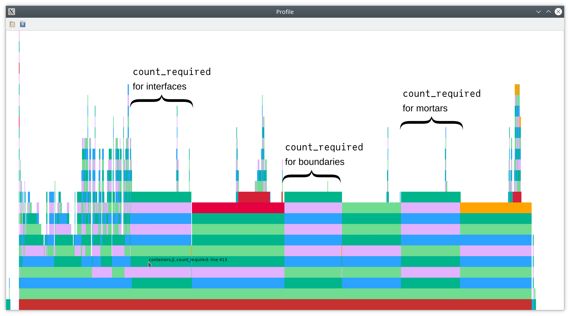
Further inspection shows that a considerable amount of time is spent inside of count_required. Indeed, this function is called three times to count the required number of interfaces, boundaries, and mortars. Since most time is spent inside C (which we cannot analyze further here using the tools we have so far), it appears to be useful to merge these three functions into a single function performing all counting operations. Thus, we will save the cost of iterating over the p4est mesh several times. Hence, we create the combined function

# Iterate over all interfaces and count
# - (inner) interfaces
# - mortars
# - boundaries
# and collect the numbers in `user_data` in this order.
function count_surfaces_iter_face(info, user_data)
  if info.sides.elem_count == 2
    # Two neighboring elements => Interface or mortar

    # Extract surface data
    sides = (load_sc_array(p4est_iter_face_side_t, info.sides, 1),
             load_sc_array(p4est_iter_face_side_t, info.sides, 2))

    if sides[1].is_hanging == 0 && sides[2].is_hanging == 0
      # No hanging nodes => normal interface
      # Unpack user_data = [interface_count] and increment interface_count
      ptr = Ptr{Int}(user_data)
      id = unsafe_load(ptr, 1)
      unsafe_store!(ptr, id + 1, 1)
    else
      # Hanging nodes => mortar
      # Unpack user_data = [mortar_count] and increment mortar_count
      ptr = Ptr{Int}(user_data)
      id = unsafe_load(ptr, 2)
      unsafe_store!(ptr, id + 1, 2)
    end
  elseif info.sides.elem_count == 1
    # One neighboring elements => Boundary

    # Unpack user_data = [boundary_count] and increment boundary_count
    ptr = Ptr{Int}(user_data)
    id = unsafe_load(ptr, 3)
    unsafe_store!(ptr, id + 1, 3)
  end

  return nothing
end

function count_required_surfaces(mesh::P4estMesh)
  # Let p4est iterate over all interfaces and call count_surfaces_iter_face
  iter_face_c = @cfunction(count_surfaces_iter_face, Cvoid, (Ptr{p4est_iter_face_info_t}, Ptr{Cvoid}))

  # interfaces, mortars, boundaries
  user_data = [0, 0, 0]

  iterate_faces(mesh, iter_face_c, user_data)

  # Return counters
  return (interfaces = user_data[1],
          mortars    = user_data[2],
          boundaries = user_data[3])
end

and modify reinitialize_containers! to

function reinitialize_containers!(mesh::P4estMesh, equations, dg::DGSEM, cache)
  # Re-initialize elements container
  @unpack elements = cache
  resize!(elements, ncells(mesh))
  init_elements!(elements, mesh, dg.basis)

  required = count_required_surfaces(mesh)

  # re-initialize interfaces container
  @unpack interfaces = cache
  resize!(interfaces, required.interfaces)
  init_interfaces!(interfaces, mesh)

  # re-initialize boundaries container
  @unpack boundaries = cache
  resize!(boundaries, required.boundaries)
  init_boundaries!(boundaries, mesh)

  # re-initialize mortars container
  @unpack mortars = cache
  resize!(mortars, required.mortars)
  init_mortars!(mortars, mesh)
end

Let’s see what we get from this.

julia> @benchmark Trixi.reinitialize_containers!($mesh, $equations, $solver, $(semi.cache))
samples: 10000; evals/sample: 1; memory estimate: 60.36 KiB; allocs estimate: 1922
ns

 (403000.0 - 419000.0]  ██████████████████████████████ 8931
 (419000.0 - 435000.0]  █▊499
 (435000.0 - 451000.0]  █▎369
 (451000.0 - 467000.0]  ▌118
 (467000.0 - 483000.0]  ▎38
 (483000.0 - 499000.0]  ▏13
 (499000.0 - 515000.0]  ▏8
 (515000.0 - 531000.0]  ▏9
 (531000.0 - 547000.0]  ▏1
 (547000.0 - 563000.0]  ▏2
 (563000.0 - 578000.0]   0
 (578000.0 - 594000.0]  ▏1
 (594000.0 - 610000.0]   0
 (610000.0 - 626000.0]  ▏1
 (626000.0 - 1.1291e7]  ▏10

                  Counts

min: 402.560 μs (0.00% GC); mean: 417.274 μs (1.78% GC); median: 405.770 μs (0.00% GC); max: 11.291 ms (95.63% GC).

That’s a nice speed-up of ca. 25%!

Step 9: Capitalizing on what we have learned

We have seen that there is some overhead of iterating over the mesh several times. Thus, we could reduce the runtime by reducing the number of mesh iterations for counting the required numbers of interfaces, mortars, and boundaries. Well, let’s do the same for the initialization step that comes next!

Instead of calling init_interfaces!, init_mortars!, and init_boundaries! separately in reinitialize_containers!, we will create a function init_surfaces! that fuses these three iterations over the mesh in p4est.

function reinitialize_containers!(mesh::P4estMesh, equations, dg::DGSEM, cache)
  # Re-initialize elements container
  @unpack elements = cache
  resize!(elements, ncells(mesh))
  init_elements!(elements, mesh, dg.basis)

  required = count_required_surfaces(mesh)

  # resize interfaces container
  @unpack interfaces = cache
  resize!(interfaces, required.interfaces)

  # resize boundaries container
  @unpack boundaries = cache
  resize!(boundaries, required.boundaries)

  # resize mortars container
  @unpack mortars = cache
  resize!(mortars, required.mortars)

  # re-initialize containers together to reduce
  # the number of iterations over the mesh in
  # p4est
  init_surfaces!(interfaces, mortars, boundaries, mesh)
end

First, we need to create a new struct that will hold our user data.

# A helper struct used in initialization methods below
mutable struct InitSurfacesIterFaceUserData{Interfaces, Mortars, Boundaries, Mesh}
  interfaces  ::Interfaces
  interface_id::Int
  mortars     ::Mortars
  mortar_id   ::Int
  boundaries  ::Boundaries
  boundary_id ::Int
  mesh        ::Mesh
end

function InitSurfacesIterFaceUserData(interfaces, mortars, boundaries, mesh)
  return InitSurfacesIterFaceUserData{
    typeof(interfaces), typeof(mortars), typeof(boundaries), typeof(mesh)}(
      interfaces, 1, mortars, 1, boundaries, 1, mesh)
end

Here, we have also written a convenience constructor initializing the counters for the different surface types to unity.

Next, we write a single function that will perform the initialization of all three different surface types together.

function init_surfaces_iter_face(info, user_data)
  # Unpack user_data
  data = unsafe_pointer_to_objref(Ptr{InitSurfacesIterFaceUserData}(user_data))

  # Function barrier because the unpacked user_data above is type-unstable
  init_surfaces_iter_face_inner(info, data)
end

# Function barrier for type stability
function init_surfaces_iter_face_inner(info, user_data)
  @unpack interfaces, mortars, boundaries = user_data

  if info.sides.elem_count == 2
    # Two neighboring elements => Interface or mortar

    # Extract surface data
    sides = (load_sc_array(p4est_iter_face_side_t, info.sides, 1),
             load_sc_array(p4est_iter_face_side_t, info.sides, 2))

    if sides[1].is_hanging == 0 && sides[2].is_hanging == 0
      # No hanging nodes => normal interface
      if interfaces !== nothing
        init_interfaces_iter_face_inner(info, sides, user_data)
      end
    else
      # Hanging nodes => mortar
      if mortars !== nothing
        init_mortars_iter_face_inner(info, sides, user_data)
      end
    end
  elseif info.sides.elem_count == 1
    # One neighboring elements => boundary
    if boundaries !== nothing
      init_boundaries_iter_face_inner(info, user_data)
    end
  end

  return nothing
end

function init_surfaces!(interfaces, mortars, boundaries, mesh::P4estMesh)
  # Let p4est iterate over all interfaces and call init_surfaces_iter_face
  iter_face_c = @cfunction(init_surfaces_iter_face,
                           Cvoid, (Ptr{p4est_iter_face_info_t}, Ptr{Cvoid}))
  user_data = InitSurfacesIterFaceUserData(
    interfaces, mortars, boundaries, mesh)

  iterate_faces(mesh, iter_face_c, user_data)

  return interfaces
end

This follows basically the same logic as count_surfaces_iter_face above to decide which type of surface we have to deal with. Note that we added some check of the form if interfaces !== nothing. These will allow us to pass interfaces = nothing in InitSurfacesIterFaceUserData to mimic what we had before in init_interfaces!, e.g.

function init_interfaces!(interfaces, mesh::P4estMesh)
  # Let p4est iterate over all interfaces and call init_surfaces_iter_face
  iter_face_c = @cfunction(init_surfaces_iter_face,
                           Cvoid, (Ptr{p4est_iter_face_info_t}, Ptr{Cvoid}))
  user_data = InitSurfacesIterFaceUserData(
    interfaces,
    nothing, # mortars
    nothing, # boundaries
    mesh)

  iterate_faces(mesh, iter_face_c, user_data)

  return interfaces
end

Finally, we need to change the first few lines of the inner initialization functions to account for the new type of user_data, e.g.

function init_interfaces_iter_face_inner(info, sides, user_data)
  @unpack interfaces, interface_id, mesh = user_data
  user_data.interface_id += 1

  # remaining part as before

That’s it. Let’s see how the new version performs.

julia> @benchmark Trixi.reinitialize_containers!($mesh, $equations, $solver, $(semi.cache))
samples: 10000; evals/sample: 1; memory estimate: 33.08 KiB; allocs estimate: 1048
ns

 (272000.0 - 297000.0]  ██████████████████████████████ 9290
 (297000.0 - 322000.0]  █▋465
 (322000.0 - 347000.0]  ▍88
 (347000.0 - 373000.0]  ▏26
 (373000.0 - 398000.0]  ▏14
 (398000.0 - 423000.0]  ▏5
 (423000.0 - 448000.0]  ▏5
 (448000.0 - 473000.0]  ▏4
 (473000.0 - 499000.0]  ▏2
 (499000.0 - 524000.0]  ▏5
 (524000.0 - 549000.0]  ▏23
 (549000.0 - 574000.0]  ▎53
 (574000.0 - 599000.0]  ▏4
 (599000.0 - 624000.0]  ▏6
 (624000.0 - 9.027e6 ]  ▏10

                  Counts

min: 271.808 μs (0.00% GC); mean: 284.722 μs (1.20% GC); median: 275.231 μs (0.00% GC); max: 9.027 ms (96.83% GC).

That’s a nice speed-up of ca. one third!

Summary and conclusions

Let’s compare our final result with the initial state.

julia> trixi_include(joinpath(examples_dir(), "2d", "elixir_advection_amr.jl"),
          mesh=P4estMesh((1, 1), polydeg=3,
                  coordinates_min=coordinates_min, coordinates_max=coordinates_max,
                  initial_refinement_level=4))
[...]
 ────────────────────────────────────────────────────────────────────────────────────
               Trixi.jl                      Time                   Allocations
                                     ──────────────────────   ───────────────────────
          Tot / % measured:               485ms / 98.3%           82.3MiB / 100%

 Section                     ncalls     time   %tot     avg     alloc   %tot      avg
 ────────────────────────────────────────────────────────────────────────────────────
 rhs!                         1.61k    208ms  43.7%   130μs   53.5MiB  65.2%  34.1KiB
[...]
 AMR                             64   72.8ms  15.3%  1.14ms   25.8MiB  31.4%   412KiB
   refine                        64   32.1ms  6.75%   502μs   5.95MiB  7.24%  95.1KiB
     solver                      64   20.5ms  4.31%   321μs   5.44MiB  6.63%  87.1KiB
     mesh                        64   11.6ms  2.43%   181μs    515KiB  0.61%  8.05KiB
       rebalance                128   10.6ms  2.22%  82.7μs   2.00KiB  0.00%    16.0B
       refine                    64    547μs  0.11%  8.55μs     0.00B  0.00%    0.00B
       ~mesh~                    64    452μs  0.09%  7.07μs    513KiB  0.61%  8.02KiB
     ~refine~                    64   26.9μs  0.01%   421ns   1.66KiB  0.00%    26.5B
   coarsen                       64   31.4ms  6.59%   490μs   7.36MiB  8.97%   118KiB
     solver                      64   19.7ms  4.13%   308μs   5.55MiB  6.76%  88.8KiB
     mesh                        64   11.7ms  2.45%   182μs   1.81MiB  2.21%  29.0KiB
       rebalance                128   10.1ms  2.12%  79.0μs   2.00KiB  0.00%    16.0B
       ~mesh~                    64   1.06ms  0.22%  16.5μs   1.29MiB  1.57%  20.6KiB
       coarsen!                  64    489μs  0.10%  7.65μs    534KiB  0.63%  8.34KiB
     ~coarsen~                   64   30.0μs  0.01%   469ns   1.66KiB  0.00%    26.5B
   indicator                     64   9.05ms  1.90%   141μs   12.4MiB  15.2%   199KiB
   ~AMR~                         64    201μs  0.04%  3.14μs   2.48KiB  0.00%    39.8B
[...]

For comparison, here are the numbers we had at the beginning.

[...]
 AMR                             64    213ms  31.2%  3.33ms    121MiB  67.7%  1.89MiB
   coarsen                       64    110ms  16.2%  1.72ms   53.9MiB  30.1%   862KiB
     solver                      64   97.4ms  14.3%  1.52ms   52.1MiB  29.1%   833KiB
     mesh                        64   12.9ms  1.90%   202μs   1.81MiB  1.01%  29.0KiB
       rebalance                128   11.2ms  1.64%  87.3μs   2.00KiB  0.00%    16.0B
       ~mesh~                    64   1.18ms  0.17%  18.4μs   1.29MiB  0.72%  20.6KiB
       coarsen!                  64    590μs  0.09%  9.22μs    534KiB  0.29%  8.34KiB
     ~coarsen~                   64   39.0μs  0.01%   609ns   1.66KiB  0.00%    26.5B
   refine                        64   91.8ms  13.4%  1.43ms   54.7MiB  30.6%   875KiB
     solver                      64   79.3ms  11.6%  1.24ms   54.2MiB  30.3%   867KiB
     mesh                        64   12.5ms  1.83%   195μs    515KiB  0.28%  8.05KiB
       rebalance                128   11.4ms  1.67%  88.9μs   2.00KiB  0.00%    16.0B
       refine                    64    613μs  0.09%  9.58μs     0.00B  0.00%    0.00B
       ~mesh~                    64    476μs  0.07%  7.44μs    513KiB  0.28%  8.02KiB
     ~refine~                    64   36.6μs  0.01%   572ns   1.66KiB  0.00%    26.5B
   indicator                     64   10.8ms  1.58%   168μs   12.4MiB  6.96%   199KiB
   ~AMR~                         64    252μs  0.04%  3.94μs   2.48KiB  0.00%    39.8B
[...]

Thus, we could reduce the runtime spend in AMR routines by ca. two thirds in total. Citing Erik Faulhaber from Issue #627:

rhs! is expected to be slower since P4estMesh is treated as a curved mesh. AMR is also expected to be slower because the curved data structures that need to be rebuilt are a lot more complex than the ones used by TreeMesh. However, AMR with P4estMesh can most likely be optimized to be at least twice as fast as it is now.

It looks like he was completely right. We even got a better speed-up of 3x instead of 2x he set as goal for us!

Let’s recapitulate some lessons that we learned.

• Profiling is an important tool to gather knowledge about the problem. Without it, we do not know which parts of our code are expensive and might optimize code that is totally irrelevant.
• Having CI tests is absolutely necesary for making sure that refactoring code doesn’t break anything and detecting possible bugs.
• We used two types of optimizations:
  1. Algorithmic improvements such as reducing the number of iterations over the p4est mesh
  2. Low-lever performance improvements such as rewriting broadcasting operations on views into loops annotated with @turbo

  Algorithmic optimizations are often harder to detect since a broader overview over the problem is necessary. However, they often provide better opportunities for improving the performance than low-lever optimizations.

• LoopVectorization.jl is a great package to improve the performance of CPU code in Julia. However, you need to know what you are doing and might run into interesting bugs. Luckily, Chris Elrod, the developer of LoopVectorization.jl, is really nice and helpful. In my experience, he will fix bugs quite fast when you report them on GitHub and provide minimal working examples (MWEs).
• Providing generic Julia code as callback via C can be tricky and we still have some type instabilities left for the future. We could fix them by passing Julia closures to C, but that’s not supported on all platforms such as ARM. Since there are ARM clusters, using this feature is not an option for us in Trixi.jl. Thus, we need to do something else to fix the type instabilities visible as red blocks at the top of the final flamegraph below.

That’s it for today! I hope you enjoyed this blog post and could learn something. Feel free to get into contact if you liked this and, say, want to contribute to Trixi.jl.

As all code published in this blog, new code developed here is released under the terms of the MIT license. Code excerpts of Trixi.jl are subject to the MIT license distributed with Trixi.