
Optimizing Julia code: Improving the performance of entropy-conservative DG methods in Trixi.jl
If you have followed my blog or my publications, you will have noticed that I’m
a principal developer of Trixi.jl,
an open source framework of high-order methods for hyperbolic conservation laws
written in Julia.
A few days ago, Andrew Winters ran some
tests to compare Trixi.jl with the HPC Fortran code
Fluxo, which also implements
discontinuous Galerkin spectral element methods (DGSEM) for hyperbolic or
hyperbolic-parabolic conservation laws.
These benchmarks compared the serial performance of Trixi.jl and Fluxo for
entropy-conservative (EC) methods for the compressible Euler equations in three
space dimensions. The mesh used for this comparison was logically Cartesian.
While Trixi has a Cartesian TreeMesh, Fluxo only implements a more general
unstructured curvilinear mesh. Thus, Andrew Winters checked also the performance
of the structured curvilinear mesh we have in Trixi.jl. At the time of writing,
this is declared as an experimental feature of Trixi.jl but will stabilize soon;
an unstructured, curvilinear mesh based on pest will be added soon.
These preliminary performance comparisons showed that
- Trixi.jl using its Cartesian mesh is faster than Fluxo using its curvilinear mesh (between 1.7x and 2.5x)
- Trixi.jl using its curvilinear mesh is slower than Fluxo using its curvilinear mesh (between 8% and 33%)
The first result is already quite nice for Trixi.jl. In particular, it demonstrates that Julia as a high-level programming language is not too far off and can be used for serious number crunching in scientific computing. However, you can imagine that I didn’t like the second result. Since I feel responsible for the serial performance of Trixi.jl, I was nerd-sniped to do something.
Since I shouldn’t be the only one being able to improve the performance of Trixi.jl, I would like to share my experience. Thus, I ended up writing another blog post about writing efficient code in Julia, my favorite programming language so far. As before, this blog post is basically a recording of the steps I made to improve the performance of a particular application of Trixi.jl. It is not designed as an introduction to Julia in general or the numerical methods we use. I will also not necessarily introduce all concepts in a pedagogically optimal way.
Our usual development workflow consists of the two steps
- Make it work
- Make it fast
Note that the first step includes adding tests and continuous integration, so that we can refactor or rewrite code later without worrying about introducing bugs or regressions. This step is absolutely necessary for any code you want to rely on! Armed with this background, we can take another stab at the second step and improve the performance.
You can find a complete set of commits and all the code in the branch
hr/blog_ec_performance
in my fork of Trixi.jl and the associated
PR #643.
Step 0: Start a Julia REPL and load some packages
All results shown below are obtained using Julia v1.6.1 and command line flags
julia --threads=1 --check-bounds=no. You can find a complete set of commits
and all the code in the branch
hr/blog_ec_performance
in my fork of Trixi.jl.
Let’s start by loading some standard packages I use when developing Julia code.
julia> using BenchmarkHistograms, ProfileView; using Revise, Trixi
BenchmarkHistograms.jl is basically a wrapper of BenchmarkTools.jl that prints benchmark results as histograms, providing more detailed information about the performance of a piece of code. ProfileView.jl allows us to profile code and visualize the results. Finally, Revise.jl makes editing Julia packages much more comfortable by re-loading modified code on the fly. If you’re not familiar with these packages, I highly recommend taking a look at them.
Next, we run some code to set up data structures we will use for benchmarking. The result shown below is obtained after running the command twice to exclude compilation time.
julia> include(joinpath(examples_dir(), "3d", "elixir_euler_ec.jl"))
[...]
 ──────────────────────────────────────────────────────────────────────────────────
              Trixi.jl                     Time                   Allocations
                                   ──────────────────────   ───────────────────────
         Tot / % measured:              325ms / 96.2%           10.1MiB / 87.5%

 Section                   ncalls     time   %tot     avg     alloc   %tot      avg
 ──────────────────────────────────────────────────────────────────────────────────
 rhs!                          56    273ms  87.4%  4.88ms   30.6KiB  0.34%     560B
   volume integral             56    212ms  67.7%  3.78ms     0.00B  0.00%    0.00B
   interface flux              56   39.8ms  12.7%   710μs     0.00B  0.00%    0.00B
   surface integral            56   9.57ms  3.06%   171μs     0.00B  0.00%    0.00B
   prolong2interfaces          56   8.60ms  2.75%   154μs     0.00B  0.00%    0.00B
   reset ∂u/∂t                 56   1.79ms  0.57%  31.9μs     0.00B  0.00%    0.00B
   Jacobian                    56   1.55ms  0.50%  27.7μs     0.00B  0.00%    0.00B
   ~rhs!~                      56    259μs  0.08%  4.62μs   30.6KiB  0.34%     560B
   prolong2mortars             56   13.4μs  0.00%   239ns     0.00B  0.00%    0.00B
   prolong2boundaries          56   11.1μs  0.00%   199ns     0.00B  0.00%    0.00B
   mortar flux                 56   10.6μs  0.00%   189ns     0.00B  0.00%    0.00B
   source terms                56   1.08μs  0.00%  19.3ns     0.00B  0.00%    0.00B
   boundary flux               56   1.07μs  0.00%  19.1ns     0.00B  0.00%    0.00B
 analyze solution               2   26.1ms  8.34%  13.0ms   34.5KiB  0.38%  17.3KiB
 I/O                            5   8.97ms  2.87%  1.79ms   8.82MiB  99.3%  1.76MiB
   save solution                2   6.15ms  1.97%  3.07ms   7.52MiB  84.6%  3.76MiB
   ~I/O~                        5   2.80ms  0.90%   560μs   1.30MiB  14.6%   266KiB
   get element variables        2   18.2μs  0.01%  9.09μs   5.50KiB  0.06%  2.75KiB
   save mesh                    2    155ns  0.00%  77.5ns     0.00B  0.00%    0.00B
 calculate dt                  12   4.39ms  1.40%   366μs     0.00B  0.00%    0.00B
 ──────────────────────────────────────────────────────────────────────────────────
We can already see that the most expensive part is the evaluation of the volume terms/integral, which is expected for such a high-order entropy-conservative DG method.
Step 1: Profile the expensive parts
The next step is to gather more information. Before trying to do some premature optimizations, we need to know where most time is spend. It won’t help us if we improve the performance of a part that only takes a few percent of the total run time. Thus, we need to profile the function that we want to optimize.
julia> function doit(n, du, u, semi)
           for _ in 1:n
               Trixi.rhs!(du, u, semi, 0.0)
           end
       end
doit (generic function with 1 method)

julia> @profview doit(10^3, similar(ode.u0), copy(ode.u0), semi)
This yields the flamegraph below (module annotations).
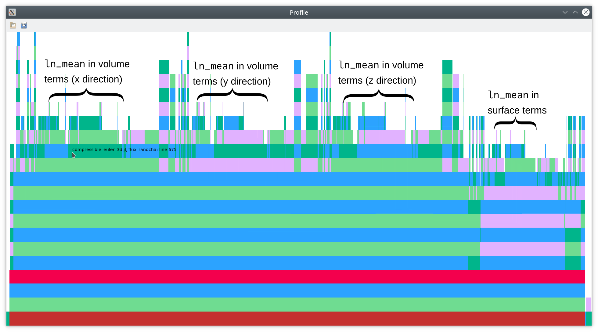
As you can see there, nearly half of the total time is spent in calculations
of the logarithmic mean ln_mean, which is a key ingredient of modern
entropy-conservative (EC) numerical fluxes for the compressible Euler equations
(and related physical models such as the MHD equations). Since the logarithmic mean
ln_mean(a, b) = (a - b) / (log(a) - log(b))
has a removable singularity at a == b, some care must be taken to implement it
correctly without problems or loss of accuracy when a ≈ b. In the context of
EC fluxes, most implementations of the logarithmic mean will probably use the
procedure described by Ismail and Roe1.
Before performing any optimizations, let’s gather some baseline benchmark results.
julia> begin
           redirect_stdout(devnull) do
               include(joinpath(examples_dir(), "3d", "elixir_euler_ec.jl"))
           end
           u_ode = copy(sol.u[1])
           du_ode = similar(u_ode)
           @benchmark Trixi.rhs!($du_ode, $u_ode, $semi, $0.0)
       end
samples: 1131; evals/sample: 1; memory estimate: 368 bytes; allocs estimate: 6
ns

 (4.338e6 - 4.406e6]  ██████████████████████████████ 707
 (4.406e6 - 4.475e6]  ███████████▌271
 (4.475e6 - 4.543e6]  ██▉66
 (4.543e6 - 4.612e6]  █▏25
 (4.612e6 - 4.68e6 ]  █▎27
 (4.68e6  - 4.749e6]  █▎27
 (4.749e6 - 4.818e6]  ▏2
 (4.818e6 - 4.886e6]  ▏2
 (4.886e6 - 4.955e6]   0
 (4.955e6 - 5.023e6]  ▏1
 (5.023e6 - 5.092e6]  ▏1
 (5.092e6 - 5.16e6 ]  ▏2

                  Counts

min: 4.338 ms (0.00% GC); mean: 4.417 ms (0.00% GC); median: 4.389 ms (0.00% GC); max: 5.160 ms (0.00% GC).
Step 2: Investigating the logarithmic mean in Fluxo (Fortran) and Trixi (Julia)
I don’t know a similarly simple way to profile the Fortran code of Fluxo. However, let’s assume that the logarithmic mean is still an expensive part there, too. Based on this hypothesis, the logical next step is to investigate the logarithmic mean in more detail.
The Julia code for the logarithmic mean used in Trixi is
function ln_mean(value1, value2)
  epsilon_f2 = 1.0e-4
  ratio = value2 / value1
  # f2 = f^2
  f2 = (ratio * (ratio - 2) + 1) / (ratio * (ratio + 2) + 1)
  if f2 < epsilon_f2
    return (value1 + value2) * 52.5 / (105 + f2 * (35 + f2 * (21 + f2 * 15)))
  else
    return (value2 - value1) / log(ratio)
  end
end
The corresponding Fortran code for the logarithmic mean used in Fluxo is
PURE FUNCTION LN_MEAN(aL,aR)
! MODULES
IMPLICIT NONE
!---------------------------------------------------------------------------------------------------
! INPUT VARIABLES
REAL,INTENT(IN) :: aL  !< left value
REAL,INTENT(IN) :: aR  !< right value
!---------------------------------------------------------------------------------------------------
! INPUT / OUTPUT VARIABLES
REAL            :: LN_MEAN  !< result
!---------------------------------------------------------------------------------------------------
! LOCaR VaLIABLES
REAL           :: Xi,u
REAL,PARAMETER :: eps=1.0E-4  ! tolerance for f^2, such that switch is smooth in double precision
!===================================================================================================
Xi = aR/aL
u=(Xi*(Xi-2.)+1.)/(Xi*(Xi+2.)+1.) !u=f^2, f=(aR-aL)/(aR+aL)=(xi-1)/(xi+1)
LN_MEAN=MERGE((aL+aR)*52.5d0/(105.d0 + u*(35.d0 + u*(21.d0 +u*15.d0))), & !u <eps (test true)
              (aR-aL)/LOG(Xi)                                         , & !u>=eps (test false)
              (u.LT.eps)                                              )   !test
END FUNCTION LN_MEAN
This looks quite similar. Why should there be a significant performance difference?
Well, what gets executed on a CPU is not the source code written in some programming language but the machine code produced by a compiler. Thus, if we want to understand performance differences of similarly looking code in different languages, we should also look at the corresponding compiled versions. This is easy to do in Julia due to the great introspection possibilities:
julia> @code_native debuginfo=:none syntax=:intel Trixi.ln_mean(0.9, 1.1)
        .text
        push    rax
        vmovapd xmm2, xmm0
        vdivsd  xmm0, xmm1, xmm0
        vmovddup        xmm3, xmm0                      # xmm3 = xmm0[0,0]
        movabs  rax, offset .rodata.cst16
        vaddpd  xmm4, xmm3, xmmword ptr [rax]
        vmulpd  xmm3, xmm3, xmm4
        movabs  rax, 139804213080288
        vaddpd  xmm3, xmm3, xmmword ptr [rax]
        vpermilpd       xmm4, xmm3, 1           # xmm4 = xmm3[1,0]
        vdivsd  xmm3, xmm3, xmm4
        movabs  rax, offset .rodata.cst8
        vmovsd  xmm4, qword ptr [rax]           # xmm4 = mem[0],zero
        vucomisd        xmm4, xmm3
        ja      L107
        vsubsd  xmm1, xmm1, xmm2
        vmovsd  qword ptr [rsp], xmm1
        movabs  rax, offset log
        call    rax
        vmovsd  xmm1, qword ptr [rsp]           # xmm1 = mem[0],zero
        vdivsd  xmm0, xmm1, xmm0
        pop     rax
        ret
L107:
        vaddsd  xmm0, xmm2, xmm1
        movabs  rax, 139804213080312
        vmulsd  xmm0, xmm0, qword ptr [rax]
        movabs  rax, 139804213080320
        vmulsd  xmm1, xmm3, qword ptr [rax]
        movabs  rax, 139804213080328
        vaddsd  xmm1, xmm1, qword ptr [rax]
        vmulsd  xmm1, xmm3, xmm1
        movabs  rax, 139804213080336
        vaddsd  xmm1, xmm1, qword ptr [rax]
        vmulsd  xmm1, xmm3, xmm1
        movabs  rax, 139804213080344
        vaddsd  xmm1, xmm1, qword ptr [rax]
        vdivsd  xmm0, xmm0, xmm1
        pop     rax
        ret
        nop     word ptr cs:[rax + rax]
The easiest way to do something similar in Fortran is to use godbolt.org, resulting in
ln_mean_:
        vmovsd  xmm1, QWORD PTR [rsi]
        vmovsd  xmm4, QWORD PTR [rdi]
        vmovsd  xmm2, QWORD PTR .LC0[rip]
        vmovsd  xmm5, QWORD PTR .LC1[rip]
        vdivsd  xmm3, xmm1, xmm4
        vsubsd  xmm0, xmm3, xmm2
        vaddsd  xmm2, xmm3, xmm2
        vfmadd132sd     xmm0, xmm5, xmm3
        vfmadd132sd     xmm2, xmm5, xmm3
        vdivsd  xmm0, xmm0, xmm2
        vmovsd  xmm2, QWORD PTR .LC2[rip]
        vcomisd xmm2, xmm0
        jbe     .L6
        vmovsd  xmm2, QWORD PTR .LC3[rip]
        vfmadd213sd     xmm2, xmm0, QWORD PTR .LC4[rip]
        vfmadd213sd     xmm2, xmm0, QWORD PTR .LC5[rip]
        vfmadd213sd     xmm2, xmm0, QWORD PTR .LC6[rip]
        vaddsd  xmm0, xmm1, xmm4
        vmulsd  xmm0, xmm0, QWORD PTR .LC7[rip]
        vdivsd  xmm0, xmm0, xmm2
        ret
.L6:
        sub     rsp, 24
        vmovsd  xmm0, xmm3, xmm3
        vmovsd  QWORD PTR [rsp+8], xmm4
        vmovsd  QWORD PTR [rsp], xmm1
        call    log
        vmovsd  xmm1, QWORD PTR [rsp]
        vmovsd  xmm4, QWORD PTR [rsp+8]
        add     rsp, 24
        vmovsd  xmm2, xmm0, xmm0
        vsubsd  xmm0, xmm1, xmm4
        vdivsd  xmm0, xmm0, xmm2
        ret
If you can’t read assembly code, you might want to read up on it a bit.
What’s important here is that the Fortran compiler produced
fused multiply-add (FMA)
instructions (vfmadd132sd and vfmadd213sd),
which combine a multiplication and an addition of floating point
numbers in a single instruction. Such FMA instructions are extremely important
and received quite some attention on modern hardware since they are responsible
for peak performance of matrix multiplication (variants of gemm in BLAS),
which are used in many contexts such as machine learning etc. Hence, we need to
make use FMA whenever possible to achieve top performance on modern hardware.
Let’s turn to a simpler example to demonstrate the compiler differences. At first, we let gfortran compile
PURE FUNCTION FOO(a,b,c)
REAL*8,INTENT(IN) :: a
REAL*8,INTENT(IN) :: b
REAL*8,INTENT(IN) :: c
REAL*8            :: FOO  !< result
FOO = a + b * c
END FUNCTION FOO
foo_:
        vmovsd  xmm0, QWORD PTR [rsi]
        vmovsd  xmm1, QWORD PTR [rdi]
        vfmadd132sd     xmm0, xmm1, QWORD PTR [rdx]
        ret
Next, let’s use gcc to compile the C code
double foo(double a, double b, double c) {
    return a * b + c;
}
to the following assembly code
foo(double, double, double):
        vfmadd132sd     xmm0, xmm2, xmm1
        ret
Finally, we check what the Julia compiler produces for a similar function:
julia> foo(a, b, c) = a * b + c
foo (generic function with 1 method)

julia> @code_native debuginfo=:none syntax=:intel foo(1.0, 2.0, 3.0)
        .text
        vmulsd  xmm0, xmm0, xmm1
        vaddsd  xmm0, xmm0, xmm2
        ret
        nop     dword ptr [rax]
Indeed, there is a significant difference between the results we get in traditional scientific computing languages such as Fortran/C/C++ and Julia; the compilers of traditional languages produce FMA instructions but Julia doesn’t! However, it’s not the fault of Julia; instead, you should rather blame LLVM, which is used under the hood by Julia. Indeed, throwing the same C code at LLVM that GCC turned into an FMA yields
foo(double, double, double):                              # @foo(double, double, double)
        vmulsd  xmm0, xmm0, xmm1
        vaddsd  xmm0, xmm0, xmm2
        ret
Now, you might think that Julia will never be able to compete with high-performance
code written in other languages when these are compiled with GCC, the Intel compiler,
or something similarly efficient. However, that’s not the case. Luckily for us,
Julia comes with great possibilities for code manipulation and generation by using
macros. Even better, the importance of FMAs has been recognized already quite some
time ago in the SciML ecosystem. Thus, we can use the solution developed there;
it’s time for @muladd from
MuladdMacro.jl, that we can pull into
Trixi via DiffEqBase.jl.
The Julia macro @muladd transforms an expression by rewriting operations where
FMA instructions can be used into calls to muladd, which LLVM will happily
compile into FMAs.
julia> using Trixi: @muladd

julia> @muladd foo(a, b, c) = a * b + c
foo (generic function with 1 method)

julia> @code_native debuginfo=:none syntax=:intel foo(1.0, 2.0, 3.0)
        .text
        vfmadd213sd     xmm0, xmm1, xmm2        # xmm0 = (xmm1 * xmm0) + xmm2
        ret
        nop     word ptr cs:[rax + rax]
That’s it! If you want to know more about what happened, you can use another
introspection tool of Julia: @macroexpand.
julia> @macroexpand @muladd foo(a, b, c) = a * b + c
:(foo(a, b, c) = begin
          #= REPL[11]:1 =#
          (muladd)(a, b, c)
      end)
Now, let’s use this for the logarithmic mean in Trixi. All we need to do
is adding the eight characters @muladd in front of the function definition.
@muladd function ln_mean(value1, value2)
  # same as before
end
Let’s see what we get!
julia> begin
           redirect_stdout(devnull) do
               include(joinpath(examples_dir(), "3d", "elixir_euler_ec.jl"))
           end
           u_ode = copy(sol.u[1])
           du_ode = similar(u_ode)
           @benchmark Trixi.rhs!($du_ode, $u_ode, $semi, $0.0)
       end
samples: 1198; evals/sample: 1; memory estimate: 368 bytes; allocs estimate: 6
ns

 (4.0e6  - 4.27e6]  ██████████████████████████████ 1023
 (4.27e6 - 4.54e6]  ██▌83
 (4.54e6 - 4.81e6]  █▍45
 (4.81e6 - 5.07e6]  ▍9
 (5.07e6 - 5.34e6]  ▍12
 (5.34e6 - 5.61e6]  ▍9
 (5.61e6 - 5.88e6]  ▏4
 (5.88e6 - 6.15e6]  ▏2
 (6.15e6 - 6.41e6]  ▏4
 (6.41e6 - 6.68e6]  ▏3
 (6.68e6 - 6.95e6]  ▏2
 (6.95e6 - 7.22e6]  ▏2

                  Counts

min: 4.004 ms (0.00% GC); mean: 4.169 ms (0.00% GC); median: 4.053 ms (0.00% GC); max: 7.216 ms (0.00% GC).
That’s an impressive performance speed-up of ca. 10% by just adding eight characters!
At good optimization levels, Fortran compilers are usually good at inlining. Let’s
nudge the Julia compiler to do the same by also adding @inline in front of
the definition of the logarithmic mean.
@muladd @inline function ln_mean(value1, value2)
  # same as before
end
Now, we get
julia> begin
           redirect_stdout(devnull) do
               include(joinpath(examples_dir(), "3d", "elixir_euler_ec.jl"))
           end
           u_ode = copy(sol.u[1])
           du_ode = similar(u_ode)
           @benchmark Trixi.rhs!($du_ode, $u_ode, $semi, $0.0)
       end
samples: 1295; evals/sample: 1; memory estimate: 368 bytes; allocs estimate: 6
ns

 (3.788e6 - 3.843e6]  ██████████████████████████████ 774
 (3.843e6 - 3.897e6]  ████████████▏310
 (3.897e6 - 3.951e6]  ███▌89
 (3.951e6 - 4.006e6]  ██50
 (4.006e6 - 4.06e6 ]  █25
 (4.06e6  - 4.114e6]  ▊18
 (4.114e6 - 4.169e6]  ▊17
 (4.169e6 - 4.223e6]  ▍7
 (4.223e6 - 4.277e6]  ▏2
 (4.277e6 - 4.332e6]   0
 (4.332e6 - 4.386e6]  ▏2
 (4.386e6 - 4.44e6 ]  ▏1

                  Counts

min: 3.788 ms (0.00% GC); mean: 3.859 ms (0.00% GC); median: 3.841 ms (0.00% GC); max: 4.440 ms (0.00% GC).
That’s another nice speed-up of ca. 5% by a simple change in the source code.
Step 3: Optimizing the split_form_kernel!
There will likely be many more opportunities to use FMAs in Trixi. For example,
let’s look at the 3D split_form_kernel!, which lies at the heart of the volume
terms/integral used for the EC method.
@inline function split_form_kernel!(du::AbstractArray{<:Any,5}, u,
                                    nonconservative_terms::Val{false}, equations,
                                    volume_flux, dg::DGSEM, cache,
                                    element, alpha=true)
  @unpack derivative_split = dg.basis

  # Calculate volume integral in one element
  for k in eachnode(dg), j in eachnode(dg), i in eachnode(dg)
    u_node = get_node_vars(u, equations, dg, i, j, k, element)

    # x direction
    # use consistency of the volume flux to make this evaluation cheaper
    flux1 = flux(u_node, 1, equations)
    integral_contribution = alpha * derivative_split[i, i] * flux1
    add_to_node_vars!(du, integral_contribution, equations, dg, i, j, k, element)
    # use symmetry of the volume flux for the remaining terms
    for ii in (i+1):nnodes(dg)
      u_node_ii = get_node_vars(u, equations, dg, ii, j, k, element)
      flux1 = volume_flux(u_node, u_node_ii, 1, equations)
      integral_contribution = alpha * derivative_split[i, ii] * flux1
      add_to_node_vars!(du, integral_contribution, equations, dg, i,  j, k, element)
      integral_contribution = alpha * derivative_split[ii, i] * flux1
      add_to_node_vars!(du, integral_contribution, equations, dg, ii, j, k, element)
    end

    # y direction
    # use consistency of the volume flux to make this evaluation cheaper
    flux2 = flux(u_node, 2, equations)
    integral_contribution = alpha * derivative_split[j, j] * flux2
    add_to_node_vars!(du, integral_contribution, equations, dg, i, j, k, element)
    # use symmetry of the volume flux for the remaining terms
    for jj in (j+1):nnodes(dg)
      u_node_jj = get_node_vars(u, equations, dg, i, jj, k, element)
      flux2 = volume_flux(u_node, u_node_jj, 2, equations)
      integral_contribution = alpha * derivative_split[j, jj] * flux2
      add_to_node_vars!(du, integral_contribution, equations, dg, i, j,  k, element)
      integral_contribution = alpha * derivative_split[jj, j] * flux2
      add_to_node_vars!(du, integral_contribution, equations, dg, i, jj, k, element)
    end

    # z direction
    # use consistency of the volume flux to make this evaluation cheaper
    flux3 = flux(u_node, 3, equations)
    integral_contribution = alpha * derivative_split[k, k] * flux3
    add_to_node_vars!(du, integral_contribution, equations, dg, i, j, k, element)
    # use symmetry of the volume flux for the remaining terms
    for kk in (k+1):nnodes(dg)
      u_node_kk = get_node_vars(u, equations, dg, i, j, kk, element)
      flux3 = volume_flux(u_node, u_node_kk, 3, equations)
      integral_contribution = alpha * derivative_split[k, kk] * flux3
      add_to_node_vars!(du, integral_contribution, equations, dg, i, j, k,  element)
      integral_contribution = alpha * derivative_split[kk, k] * flux3
      add_to_node_vars!(du, integral_contribution, equations, dg, i, j, kk, element)
    end
  end
end
First, we can make an algorithmic improvement by utilizing knowledge that’s not
visible from the source code. Indeed, the matrix derivative_split will be
completely skew-symmetric, meaning that its diagonal is zero. Hence, we can skip
the computation of the fluxes that are multiplied by the diagonal terms,
resulting in
@inline function split_form_kernel!(du::AbstractArray{<:Any,5}, u,
                                    nonconservative_terms::Val{false}, equations,
                                    volume_flux, dg::DGSEM, cache,
                                    element, alpha=true)
  @unpack derivative_split = dg.basis

  # Calculate volume integral in one element
  for k in eachnode(dg), j in eachnode(dg), i in eachnode(dg)
    u_node = get_node_vars(u, equations, dg, i, j, k, element)

    # x direction
    # All diagonal entries of `derivative_split` are zero. Thus, we can skip
    # the computation of the diagonal terms. In addition, we use the symmetry
    # of the `volume_flux` to save half of the possible two-poitn flux
    # computations.
    for ii in (i+1):nnodes(dg)
      u_node_ii = get_node_vars(u, equations, dg, ii, j, k, element)
      flux1 = volume_flux(u_node, u_node_ii, 1, equations)
      integral_contribution = alpha * derivative_split[i, ii] * flux1
      add_to_node_vars!(du, integral_contribution, equations, dg, i,  j, k, element)
      integral_contribution = alpha * derivative_split[ii, i] * flux1
      add_to_node_vars!(du, integral_contribution, equations, dg, ii, j, k, element)
    end

    # y direction
    for jj in (j+1):nnodes(dg)
      u_node_jj = get_node_vars(u, equations, dg, i, jj, k, element)
      flux2 = volume_flux(u_node, u_node_jj, 2, equations)
      integral_contribution = alpha * derivative_split[j, jj] * flux2
      add_to_node_vars!(du, integral_contribution, equations, dg, i, j,  k, element)
      integral_contribution = alpha * derivative_split[jj, j] * flux2
      add_to_node_vars!(du, integral_contribution, equations, dg, i, jj, k, element)
    end

    # z direction
    for kk in (k+1):nnodes(dg)
      u_node_kk = get_node_vars(u, equations, dg, i, j, kk, element)
      flux3 = volume_flux(u_node, u_node_kk, 3, equations)
      integral_contribution = alpha * derivative_split[k, kk] * flux3
      add_to_node_vars!(du, integral_contribution, equations, dg, i, j, k,  element)
      integral_contribution = alpha * derivative_split[kk, k] * flux3
      add_to_node_vars!(du, integral_contribution, equations, dg, i, j, kk, element)
    end
  end
end
After this change, we get
julia> redirect_stdout(devnull) do
           include(joinpath(examples_dir(), "3d", "elixir_euler_ec.jl"))
       end; du_ode = similar(ode.u0); u_ode = copy(ode.u0); @benchmark Trixi.rhs!($du_ode, $u_ode, $semi, $0.0)
samples: 1302; evals/sample: 1; memory estimate: 368 bytes; allocs estimate: 6
ns

 (3.675e6 - 3.737e6]  █████▍81
 (3.737e6 - 3.798e6]  ██████████████████████████▋406
 (3.798e6 - 3.86e6 ]  ██████████████████████████████ 459
 (3.86e6  - 3.922e6]  ████████████▍189
 (3.922e6 - 3.983e6]  ███▉59
 (3.983e6 - 4.045e6]  ██▍35
 (4.045e6 - 4.107e6]  ██▍36
 (4.107e6 - 4.168e6]  █▌22
 (4.168e6 - 4.23e6 ]  ▋9
 (4.23e6  - 4.292e6]  ▎3
 (4.292e6 - 4.353e6]  ▏1
 (4.353e6 - 5.46e6 ]  ▎2

                  Counts

min: 3.675 ms (0.00% GC); mean: 3.839 ms (0.00% GC); median: 3.814 ms (0.00% GC); max: 5.460 ms (0.00% GC).
This improvement of ca. 2.5% is not really substantial. Well, that’s somehow
expected, since the computation of EC volume_fluxes is much more expensive
than the computation of the common fluxes, at least for the compressible Euler
equations of gas dynamics we’re using in this example. However, the situation
can be different for other systems of conservation laws. In the end, it’s an
algorithmic improvement that we don’t want to miss.
Next, we will use more FMAs. Looking at the split_form_kernel!, opportunities
for more FMAs can be found in lines of the form
integral_contribution = alpha * derivative_split[i, ii] * flux1
add_to_node_vars!(du, integral_contribution, equations, dg, i,  j, k, element)
where we multiply a flux by some scalar and add it to du. FMAs cannot be used
for code like this since function arguments are evaluated before they are
passed, even if the function is inlined. Hence, we write a new method
@muladd @inline function add_to_node_vars!(u, factor, u_node, equations, solver::DG, indices...)
  for v in eachvariable(equations)
    u[v, indices...] = u[v, indices...] + factor * u_node[v]
  end
  return nothing
end
This method has an additional argument factor multiplying what we will add to
u at the position determined by the indices.
Next, we re-write the split_form_kernel! to use this new method of
add_to_node_vars!.
@inline function split_form_kernel!(du::AbstractArray{<:Any,5}, u,
                                    nonconservative_terms::Val{false}, equations,
                                    volume_flux, dg::DGSEM, cache,
                                    element, alpha=true)
  # true * [some floating point value] == [exactly the same floating point value]
  # This can (hopefully) be optimized away due to constant propagation.
  @unpack derivative_split = dg.basis

  # Calculate volume integral in one element
  for k in eachnode(dg), j in eachnode(dg), i in eachnode(dg)
    u_node = get_node_vars(u, equations, dg, i, j, k, element)

    # All diagonal entries of `derivative_split` are zero. Thus, we can skip
    # the computation of the diagonal terms. In addition, we use the symmetry
    # of the `volume_flux` to save half of the possible two-poitn flux
    # computations.

    # x direction
    for ii in (i+1):nnodes(dg)
      u_node_ii = get_node_vars(u, equations, dg, ii, j, k, element)
      flux1 = volume_flux(u_node, u_node_ii, 1, equations)
      add_to_node_vars!(du, alpha * derivative_split[i, ii], flux1, equations, dg, i,  j, k, element)
      add_to_node_vars!(du, alpha * derivative_split[ii, i], flux1, equations, dg, ii, j, k, element)
    end

    # y direction
    for jj in (j+1):nnodes(dg)
      u_node_jj = get_node_vars(u, equations, dg, i, jj, k, element)
      flux2 = volume_flux(u_node, u_node_jj, 2, equations)
      add_to_node_vars!(du, alpha * derivative_split[j, jj], flux2, equations, dg, i, j,  k, element)
      add_to_node_vars!(du, alpha * derivative_split[jj, j], flux2, equations, dg, i, jj, k, element)
    end

    # z direction
    for kk in (k+1):nnodes(dg)
      u_node_kk = get_node_vars(u, equations, dg, i, j, kk, element)
      flux3 = volume_flux(u_node, u_node_kk, 3, equations)
      add_to_node_vars!(du, alpha * derivative_split[k, kk], flux3, equations, dg, i, j, k,  element)
      add_to_node_vars!(du, alpha * derivative_split[kk, k], flux3, equations, dg, i, j, kk, element)
    end
  end
end
This results in
julia> begin
           redirect_stdout(devnull) do
               include(joinpath(examples_dir(), "3d", "elixir_euler_ec.jl"))
           end
           u_ode = copy(sol.u[1])
           du_ode = similar(u_ode)
           @benchmark Trixi.rhs!($du_ode, $u_ode, $semi, $0.0)
       end
samples: 1365; evals/sample: 1; memory estimate: 368 bytes; allocs estimate: 6
ns

 (3.53e6 - 3.67e6]  ██████████████████████████████ 1012
 (3.67e6 - 3.81e6]  █████▍178
 (3.81e6 - 3.95e6]  ██▉93
 (3.95e6 - 4.08e6]  █▎40
 (4.08e6 - 4.22e6]  ▋17
 (4.22e6 - 4.36e6]  ▎7
 (4.36e6 - 4.49e6]  ▏3
 (4.49e6 - 4.63e6]  ▎5
 (4.63e6 - 4.77e6]  ▎6
 (4.77e6 - 4.91e6]  ▏2
 (4.91e6 - 5.04e6]   0
 (5.04e6 - 5.39e6]  ▏2

                  Counts

min: 3.534 ms (0.00% GC); mean: 3.660 ms (0.00% GC); median: 3.588 ms (0.00% GC); max: 5.389 ms (0.00% GC).
That’s another nice speed-up of ca. 5%.
Of course, we have also implemented the same optimizations for similar
split_form_kernel!s in other dimensions and curvilinear meshes.
Step 4: More FMAs
To enable FMAs systematically throughout Trixi, we run the following code.
julia> function muladd_file(filename)
           file = read(filename, String) |> strip
           startswith(file, "# By default, Julia/LLVM does not use fused multiply-add operations (FMAs).") && return nothing
           open(filename, "w") do io
               println(io, "# By default, Julia/LLVM does not use fused multiply-add operations (FMAs).")
               println(io, "# Since these FMAs can increase the performance of many numerical algorithms,")
               println(io, "# we need to opt-in explicitly.")
               println(io, "# See https://ranocha.de/blog/Optimizing_EC_Trixi for further details.")
               println(io, "@muladd begin\n\n")
               println(io, file)
               println(io, "\n\nend # @muladd")
           end
       end
muladd_file (generic function with 1 method)

julia> for (root, dirs, files) in walkdir(dirname(pathof(Trixi)))
           for file in files
               endswith(file, ".jl") || continue
               file == "interpolation.jl" && continue # uses explicit performance annotations
               filename = joinpath(root, file)
               filename == pathof(Trixi) && continue
               muladd_file(filename)
           end
       end
Let’s see what we get from this change.
julia> begin
           redirect_stdout(devnull) do
               include(joinpath(examples_dir(), "3d", "elixir_euler_ec.jl"))
           end
           u_ode = copy(sol.u[1])
           du_ode = similar(u_ode)
           @benchmark Trixi.rhs!($du_ode, $u_ode, $semi, $0.0)
       end
samples: 1427; evals/sample: 1; memory estimate: 368 bytes; allocs estimate: 6
ns

 (3.443e6 - 3.484e6]  ██████████████████████████████ 717
 (3.484e6 - 3.525e6]  ██████████████████▉449
 (3.525e6 - 3.566e6]  ████▎99
 (3.566e6 - 3.608e6]  ██▉68
 (3.608e6 - 3.649e6]  █▎29
 (3.649e6 - 3.69e6 ]  █▏26
 (3.69e6  - 3.731e6]  ▊16
 (3.731e6 - 3.772e6]  ▋12
 (3.772e6 - 3.814e6]  ▎4
 (3.814e6 - 3.855e6]  ▏2
 (3.855e6 - 3.896e6]  ▎3
 (3.896e6 - 4.092e6]  ▏2

                  Counts

min: 3.443 ms (0.00% GC); mean: 3.502 ms (0.00% GC); median: 3.484 ms (0.00% GC); max: 4.092 ms (0.00% GC).
That’s another speed-up of ca. 5%.
Step 5: Improving the logarithmic mean even more
Next, let’s revisit the logarithmic mean.
@inline function ln_mean(x, y)
  epsilon_f2 = 1.0e-4
  ratio = y / x
  f2 = (ratio * (ratio - 2) + 1) / (ratio * (ratio + 2) + 1) # f2 = f^2
  if f2 < epsilon_f2
    return (x + y) * 52.5 / (105 + f2 * (35 + f2 * (21 + f2 * 15)))
  else
    return (y - x) / log(ratio)
  end
end
If you are really interested in performance, you should know that divisions are
significantly more expensive (in terms of latency and reciprocal throughput)
than multiplications. If you want to know more about this, search for
mulsd (multiplication) and divsd (division) in the instruction table of
Fog2. Taking Intel processors of the 9th generation (“Coffee Lake”) as
an example, we have
| Latency | Reciprocal throughput | |
|---|---|---|
mulsd |
4 | 0.5 |
divsd |
13-14 | 4 |
In our code for ln_mean, we see a division ratio = y / x at the very beginning,
another division in f2 = (ratio * (ratio - 2) + 1) / (ratio * (ratio + 2) + 1)
depending on the first one, and another division later depending on the computation
of f2. Thus, we will be able to speed-up the computation by reformulating the
expression for f2 while avoiding the first division ratio = y / x. Indeed,
we have (in exact arithmetic)
f2 = (ratio^2 - 2 * ratio + 1) / (ratio^2 + 2 * ratio + 1)
   = (ratio - 1)^2 / (ratio + 1)^2
   = (y / x - 1)^2 / (y / x + 1)^2
   = (y - x)^2 / (x + y)^2
   = (x * (x - 2 * y) + y * y) / (x * (x + 2 * y) + y * y)
Inserting this last expression, we arrive at
@inline function ln_mean(x, y)
  epsilon_f2 = 1.0e-4
  f2 = (x * (x - 2 * y) + y * y) / (x * (x + 2 * y) + y * y) # f2 = f^2
  if f2 < epsilon_f2
    return (x + y) * 52.5 / (105 + f2 * (35 + f2 * (21 + f2 * 15)))
  else
    return (y - x) / log(y / x)
  end
end
Let’s see what we get from this change.
julia> begin
           redirect_stdout(devnull) do
               include(joinpath(examples_dir(), "3d", "elixir_euler_ec.jl"))
           end
           u_ode = copy(sol.u[1])
           du_ode = similar(u_ode)
           @benchmark Trixi.rhs!($du_ode, $u_ode, $semi, $0.0)
       end
samples: 1500; evals/sample: 1; memory estimate: 368 bytes; allocs estimate: 6
ns

 (3.232e6 - 3.293e6]  ██████████████████████████████ 734
 (3.293e6 - 3.355e6]  █████████████▋332
 (3.355e6 - 3.416e6]  ████████▎200
 (3.416e6 - 3.477e6]  █████▊139
 (3.477e6 - 3.538e6]  █▊42
 (3.538e6 - 3.599e6]  ▉21
 (3.599e6 - 3.661e6]  ▌10
 (3.661e6 - 3.722e6]  ▍9
 (3.722e6 - 3.783e6]  ▏2
 (3.783e6 - 3.844e6]  ▎6
 (3.844e6 - 3.905e6]  ▏1
 (3.905e6 - 3.967e6]  ▎4

                  Counts

min: 3.232 ms (0.00% GC); mean: 3.330 ms (0.00% GC); median: 3.295 ms (0.00% GC); max: 3.967 ms (0.00% GC).
That’s a nice speed-up of ca. 5% in total by optimizing the logarithmic mean!
We can get another minor performance boost by avoiding the additional
multiplication by 52.5 by dividing the coefficients in the denominator
appropriately. In addition, we use @evalpoly from Julia’s standard library
instead of writing our own version of the Horner scheme, resulting in
@inline function ln_mean(x, y)
  epsilon_f2 = 1.0e-4
  f2 = (x * (x - 2 * y) + y * y) / (x * (x + 2 * y) + y * y)
  if f2 < epsilon_f2
    return (x + y) / @evalpoly(f2, 2, 2/3, 2/5, 2/7)
  else
    return (y - x) / log(y / x)
  end
end
That looks even closer to the mathematical expression from the paper. In addition, we get
julia> begin
           redirect_stdout(devnull) do
               include(joinpath(examples_dir(), "3d", "elixir_euler_ec.jl"))
           end
           u_ode = copy(sol.u[1])
           du_ode = similar(u_ode)
           @benchmark Trixi.rhs!($du_ode, $u_ode, $semi, $0.0)
       end
samples: 1526; evals/sample: 1; memory estimate: 368 bytes; allocs estimate: 6
ns

 (3.174e6 - 3.254e6]  ██████████████████████████████▏847
 (3.254e6 - 3.334e6]  ████████████▎343
 (3.334e6 - 3.415e6]  ████████▍233
 (3.415e6 - 3.495e6]  ██▌70
 (3.495e6 - 3.576e6]  ▋16
 (3.576e6 - 3.656e6]  ▎7
 (3.656e6 - 3.736e6]  ▎5
 (3.736e6 - 3.817e6]   0
 (3.817e6 - 3.897e6]  ▏1
 (3.897e6 - 3.978e6]  ▏2
 (3.978e6 - 4.058e6]   0
 (4.058e6 - 4.386e6]  ▏2

                  Counts

min: 3.174 ms (0.00% GC); mean: 3.273 ms (0.00% GC); median: 3.242 ms (0.00% GC); max: 4.386 ms (0.00% GC).
That’s another minor speed-up of ca. 2%.
Of course, we also added an appropriate comment in the source code, explaining what we have done:
# Compute the logarithmic mean
#     ln_mean(x, y) = (y - x) / (log(y) - log(x)) = (y - x) / log(y / x)
# Problem: The formula above has a removable singularity at `x == y`. Thus,
# some care must be taken to implement it correctly without problems or loss
# of accuracy when `x ≈ y`. Here, we use the approach proposed by
# Ismail and Roe (2009).
# Set ξ = y / x. Then, we have
#     (y - x) / log(y / x) = (x + y) / log(ξ) * (ξ - 1) / (ξ + 1)
# Set f = (ξ - 1) / (ξ + 1) = (y - x) / (x + y). Then, we use the expansion
#     log(ξ) = 2 * f * (1 + f^2 / 3 + f^4 / 5 + f^6 / 7) + O(ξ^9)
# Inserting the first few terms of this expansion yields
#     (y - x) / log(ξ) ≈ (x + y) * f / (2 * f * (1 + f^2 / 3 + f^4 / 5 + f^6 / 7))
#                      = (x + y) / (2 + 2/3 * f^2 + 2/5 * f^4 + 2/7 * f^6)
#
# Since divisions are usually more expensive on modern hardware than
# multiplications (Agner Fog), we try to avoid computing two divisions. Thus,
# we use
#     f^2 = (y - x)^2 / (x + y)^2
#         = (x * (x - 2 * y) + y * y) / (x * (x + 2 * y) + y * y)
#
# Given ε = 1.0e-4, we use the following algorithm.
#     if f^2 < ε
#       # use the expansion above
#     else
#       # use the direct formula (y - x) / log(y / x)
#     end
#
# - Ismail, Roe (2009).
#   Affordable, entropy-consistent Euler flux functions II: Entropy production at shocks.
#   [DOI: 10.1016/j.jcp.2009.04.021](https://doi.org/10.1016/j.jcp.2009.04.021)
# - Agner Fog.
#   Lists of instruction latencies, throughputs and micro-operation breakdowns
#   for Intel, AMD, and VIA CPUs.
#   https://www.agner.org/optimize/instruction_tables.pdf
Step 6: Avoiding more divisions in the EC numerical flux
Let’s have another look at the EC numerical flux used in this example. It contains two lines of the form
rho_p_mean = ln_mean(rho_ll / p_ll, rho_rr / p_rr)
...
f5 = f1 * ( velocity_square_avg + 1 / ((equations.gamma-1) * rho_p_mean) ) + 0.5 * (p_ll*v1_rr + p_rr*v1_ll)
Obviously, there are some divisions that can possibly be avoided. First, we know
already that the final result of the logarithmic mean ln_mean is computed by
a division. Hence, we can save the inverse division by writing a new method
# 1 / ln_mean(x, y)
@inline function inv_ln_mean(x, y)
  epsilon_f2 = 1.0e-4
  f2 = (x * (x - 2 * y) + y * y) / (x * (x + 2 * y) + y * y) # f2 = f^2
  if f2 < epsilon_f2
    return @evalpoly(f2, 2, 2/3, 2/5, 2/7) / (x + y)
  else
    return log(y / x) / (y - x)
  end
end
Using this new method in the numerical flux results in
inv_rho_p_mean = inv_ln_mean(rho_ll / p_ll, rho_rr / p_rr)
...
f5 = f1 * ( velocity_square_avg + inv_rho_p_mean / (equations.gamma-1) ) + 0.5 * (p_ll*v1_rr + p_rr*v1_ll)
Now, we get
julia> begin
           redirect_stdout(devnull) do
               include(joinpath(examples_dir(), "3d", "elixir_euler_ec.jl"))
           end
           u_ode = copy(sol.u[1])
           du_ode = similar(u_ode)
           @benchmark Trixi.rhs!($du_ode, $u_ode, $semi, $0.0)
       end
samples: 1570; evals/sample: 1; memory estimate: 368 bytes; allocs estimate: 6
ns

 (3.019e6 - 3.099e6]  ██████████████████████████████ 648
 (3.099e6 - 3.179e6]  █████████████████▌377
 (3.179e6 - 3.259e6]  █████████▊208
 (3.259e6 - 3.339e6]  ████▊102
 (3.339e6 - 3.419e6]  ███▊79
 (3.419e6 - 3.499e6]  ██▎47
 (3.499e6 - 3.579e6]  █▋35
 (3.579e6 - 3.659e6]  █▎26
 (3.659e6 - 3.739e6]  █21
 (3.739e6 - 3.819e6]  ▉17
 (3.819e6 - 3.899e6]  ▎5
 (3.899e6 - 3.978e6]  ▎5

                  Counts

min: 3.019 ms (0.00% GC); mean: 3.182 ms (0.00% GC); median: 3.123 ms (0.00% GC); max: 3.978 ms (0.00% GC).
That’s another speed-up of ca. 4%.
We can also avoid the remaining division in the calculation of f5 by adding a
new field inv_gamma_minus_one to the compressible Euler equations.
struct CompressibleEulerEquations3D{RealT<:Real} <: AbstractCompressibleEulerEquations{3, 5}
  gamma::RealT               # ratio of specific heats
  inv_gamma_minus_one::RealT # = inv(gamma - 1); can be used to write slow divisions as fast multiplications

  function CompressibleEulerEquations3D(gamma)
    γ, inv_gamma_minus_one = promote(gamma, inv(gamma - 1))
    new{typeof(γ)}(γ, inv_gamma_minus_one)
  end
end
Then, we can use this additional information here
f5 = f1 * ( velocity_square_avg + inv_rho_p_mean * equations.inv_gamma_minus_one ) + 0.5 * (p_ll*v1_rr + p_rr*v1_ll)
Of course, we also update the other dimensions and use similar opportunities
to get some speed-up from equations.inv_gamma_minus_one.
Now, we get
julia> begin
           redirect_stdout(devnull) do
               include(joinpath(examples_dir(), "3d", "elixir_euler_ec.jl"))
           end
           u_ode = copy(sol.u[1])
           du_ode = similar(u_ode)
           @benchmark Trixi.rhs!($du_ode, $u_ode, $semi, $0.0)
       end
samples: 1675; evals/sample: 1; memory estimate: 384 bytes; allocs estimate: 6
ns

 (2.898e6 - 2.972e6]  ██████████████████████████████ 1036
 (2.972e6 - 3.046e6]  ████████▊301
 (3.046e6 - 3.12e6 ]  ██████▏211
 (3.12e6  - 3.194e6]  ██▏73
 (3.194e6 - 3.269e6]  █▏38
 (3.269e6 - 3.343e6]  ▎6
 (3.343e6 - 3.417e6]  ▎5
 (3.417e6 - 3.491e6]  ▏1
 (3.491e6 - 3.566e6]   0
 (3.566e6 - 3.64e6 ]  ▏1
 (3.64e6  - 3.714e6]  ▏1
 (3.714e6 - 3.788e6]  ▏2

                  Counts

min: 2.898 ms (0.00% GC); mean: 2.982 ms (0.00% GC); median: 2.946 ms (0.00% GC); max: 3.788 ms (0.00% GC).
That’s a nice speed-up of ca. 6%.
Finally, we can use more analytical approaches to find another opportunity for avoiding divisions. Looking at
inv_rho_p_mean = inv_ln_mean(rho_ll / p_ll, rho_rr / p_rr)
let’s insert the definition of the inverse logarithmic mean
  inv_ln_mean(rho_ll / p_ll, rho_rr / p_rr)
= log((rho_ll/p_ll) / (rho_rr/p_rr)) / (rho_ll/p_ll - rho_rr/p_rr)
= p_ll * p_rr * log((rho_ll*p_rr) / (rho_rr*p_ll)) / (rho_ll*p_rr - rho_rr*p_ll)
Hence, we can use
# Equivalent to `inv_ln_mean(rho_ll / p_ll, rho_rr / p_rr)` since
#     log((ϱₗ/pₗ) / (ϱᵣ/pᵣ)) / (ϱₗ/pₗ - ϱᵣ/pᵣ)
#   = pₗ pᵣ log((ϱₗ pᵣ) / (ϱᵣ pₗ)) / (ϱₗ pᵣ - ϱᵣ pₗ)
inv_rho_p_mean = p_ll * p_rr * inv_ln_mean(rho_ll * p_rr, rho_rr * p_ll)
Now, we get
julia> begin
           redirect_stdout(devnull) do
               include(joinpath(examples_dir(), "3d", "elixir_euler_ec.jl"))
           end
           u_ode = copy(sol.u[1])
           du_ode = similar(u_ode)
           @benchmark Trixi.rhs!($du_ode, $u_ode, $semi, $0.0)
       end
samples: 1745; evals/sample: 1; memory estimate: 384 bytes; allocs estimate: 6
ns

 (2.802e6 - 2.86e6 ]  ██████████████████████████████ 932
 (2.86e6  - 2.918e6]  ████████████████████▉645
 (2.918e6 - 2.976e6]  ███▉118
 (2.976e6 - 3.034e6]  ▉27
 (3.034e6 - 3.092e6]  ▍10
 (3.092e6 - 3.151e6]  ▎4
 (3.151e6 - 3.209e6]  ▏2
 (3.209e6 - 3.267e6]  ▏3
 (3.267e6 - 3.325e6]  ▏1
 (3.325e6 - 3.383e6]   0
 (3.383e6 - 3.441e6]  ▏1
 (3.441e6 - 3.671e6]  ▏2

                  Counts

min: 2.802 ms (0.00% GC); mean: 2.863 ms (0.00% GC); median: 2.852 ms (0.00% GC); max: 3.671 ms (0.00% GC).
That’s a another speed-up of ca. 4%.
Summary and conclusions
We developed and discussed ways to improve the performance of entropy-conservative
numerical methods for the compressible Euler equations in Trixi.jl. Together,
all of these optimizations improved the performance on the Cartesian TreeMesh
by ca. 35%. We could improve the performance on a curvilinear, structured
mesh even slightly more by ca. 38% (replace “elixir_euler_ec.jl” by
“elixir_euler_ec_curved.jl” in the benchmark code above).
Let’s recapitulate some lessons that we learned.
- FMA (fused multiply-add) instructions are key to good performance on modern hardware (when applicable).
- Divisions are more expensive on modern hardware than multiplications.
- Profiling is an important tool to gather knowledge about the problem. Without it, we do not know which parts of our code are expensive and might optimize code that is totally irrelevant.
- Having CI tests is absolutely necesary for making sure that refactoring code doesn’t break anything and detecting possible bugs.
That’s it for today! I hope you enjoyed this blog post and could learn something. Feel free to get into contact if you liked this and, say, want to contribute to Trixi.jl.
As all code published in this blog, new code developed here is released under the terms of the MIT license. Code excerpts of Trixi.jl are subject to the MIT license distributed with Trixi. Code excerpts of Fluxo are subject to the GPL license distributed with Fluxo.
References
-
Ismail, Roe (2009). Affordable, entropy-consistent Euler flux functions II: Entropy production at shocks. DOI: 10.1016/j.jcp.2009.04.021 ↩
-
Agner Fog. Lists of instruction latencies, throughputs and micro-operation breakdowns for Intel, AMD, and VIA CPUs. https://www.agner.org/optimize/instruction_tables.pdf ↩