Korteweg-de Vries equation

Let's consider the Korteweg-de Vries (KdV) equation

\[\begin{aligned} \partial_t u(t,x) + \partial_x \frac{u(t,x)^2}{2} + \partial_x^3 u(t,x) &= 0, && t \in (0,T), x \in (x_{min}, x_{max}), \\ u(0,x) &= u_0(x), && x \in (x_{min}, x_{max}), \\ \end{aligned}\]

with periodic boundary conditions. The KdV equation has the quadratic invariant

\[ J = \frac{1}{2} \int u(t,x)^2 \mathrm{d}x.\]

A classical trick to conserve this invariant is to use following split form

\[ u_t + \frac{1}{3} (u^2)_x + \frac{1}{3} u u_x + \partial_x^3 u = 0.\]

Indeed, integration by parts with periodic boundary conditions yields

\[\begin{aligned} \partial_t J &= \int u u_t = -\frac{1}{3} \int u (u^2)_x - \frac{1}{3} \int u^2 u_x - \int u \partial_x^3 u \\ &= 0 + \frac{1}{3} \int u_x u^2 - \frac{1}{3} \int u^2 u_x + 0 = 0. \end{aligned}\]

Basic example using finite difference SBP operators

Let's create an appropriate discretization of this equation step by step. At first, we load packages that we will use in this example.

using SummationByPartsOperators, OrdinaryDiffEq
using LaTeXStrings; using Plots: Plots, plot, plot!, savefig

Next, we specify the initial data as Julia function as well as the spatial domain and the time span. Here, we use an analytic soliton solution of the KdV equation for the initial data.

# traveling wave solution (soliton)
get_xmin() = 0.0  # left boundary of the domain
get_xmax() = 80.0 # right boundary of the domain
get_c() = 2 / 3   # wave speed
function usol(t, x)
    xmin = get_xmin()
    xmax = get_xmax()
    μ = (xmax - xmin) / 2
    c = get_c()
    A = 3 * c
    K = sqrt(1/c - 1)
    x_t = mod(x - c*t - xmin, xmax - xmin) + xmin - μ

    A / cosh(sqrt(3*A) / 6 * x_t)^2
end

tspan = (0.0, (get_xmax() - get_xmin()) / (3 * get_c()) + 10 * (get_xmax() - get_xmin()) / get_c())

(0.0, 1240.0)

Next, we implement the semidiscretization using the interface of OrdinaryDiffEq.jl which is part of DifferentialEquations.jl. For simplicity, we just use the out-of-place version here since we do not have to worry about appropriate temporary buffers when using automatic differentiation in implicit time integration methods.

function kdv(u, parameters, t)
    D1 = parameters.D1
    D3 = parameters.D3

    # conservative semidiscretization using a split form
    return (-1 / 3) * (u .* (D1 * u) + D1 * (u.^2)) - D3 * u
end

kdv (generic function with 1 method)

Next, we choose first- and third-derivative SBP operators D1, D3, evaluate the initial data on the grid, and set up the semidiscretization as an ODE problem.

N = 128 # number of grid points
D1 = periodic_derivative_operator(derivative_order=1, accuracy_order=8,
                                  xmin=get_xmin(), xmax=get_xmax(), N=N)
D3 = periodic_derivative_operator(derivative_order=3, accuracy_order=8,
                                  xmin=get_xmin(), xmax=get_xmax(), N=N)
u0 = usol.(first(tspan), grid(D1))
parameters = (; D1, D3)

ode = ODEProblem(kdv, u0, tspan, parameters);

ODEProblem with uType Vector{Float64} and tType Float64. In-place: false
timespan: (0.0, 1240.0)
u0: 128-element Vector{Float64}:
 5.2371088845943444e-14
 8.724018505611473e-14
 1.4532540866227717e-13
 2.4208424580109605e-13
 4.032659023947894e-13
 6.717636147537472e-13
 1.119029284219571e-12
 1.864088068240953e-12
 3.1052130405874536e-12
 5.1726890975335685e-12
 ⋮
 5.1726890975335685e-12
 3.1052130405874536e-12
 1.864088068240953e-12
 1.119029284219571e-12
 6.717636147537472e-13
 4.032659023947894e-13
 2.4208424580109605e-13
 1.4532540866227717e-13
 8.724018505611473e-14

Finally, we can solve the ODE using a Rosenbrock method with adaptive time stepping. We use such a linearly implicit time integration method since the third-order derivative makes the system stiff.

sol = solve(ode, Rodas5(), saveat=range(first(tspan), stop=last(tspan), length=200))

plot(xguide=L"x", yguide=L"u")
plot!(evaluate_coefficients(sol[1], D1), label=L"u_0")
plot!(evaluate_coefficients(sol[end], D1), label=L"u_\mathrm{numerical}")
savefig("example_kdv.png");

"/home/runner/work/SummationByPartsOperators.jl/SummationByPartsOperators.jl/docs/build/tutorials/example_kdv.png"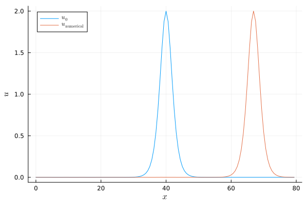

Advanced visualization

Let's create an animation of the numerical solution.

using Printf; using Plots: Animation, frame, gif

let anim = Animation()
    idx = 1
    x, u = evaluate_coefficients(sol[idx], D1)
    fig = plot(x, u, xguide=L"x", yguide=L"u", xlim=extrema(x), ylim=(-0.05, 2.05),
              label="", title=@sprintf("\$t = %6.2f \$", sol.t[idx]))
    for idx in 1:length(sol.t)
        fig[1] = x, sol.u[idx]
        plot!(title=@sprintf("\$t = %6.2f \$", sol.t[idx]))
        frame(anim)
    end
    gif(anim, "example_kdv.gif")
end

Package versions

These results were obtained using the following versions.

using InteractiveUtils
versioninfo()

using Pkg
Pkg.status(["SummationByPartsOperators", "OrdinaryDiffEq"],
           mode=PKGMODE_MANIFEST)

Julia Version 1.6.7
Commit 3b76b25b64 (2022-07-19 15:11 UTC)
Platform Info:
  OS: Linux (x86_64-pc-linux-gnu)
  CPU: AMD EPYC 7763 64-Core Processor
  WORD_SIZE: 64
  LIBM: libopenlibm
  LLVM: libLLVM-11.0.1 (ORCJIT, generic)
Environment:
  JULIA_PKG_SERVER_REGISTRY_PREFERENCE = eager
      Status `~/work/SummationByPartsOperators.jl/SummationByPartsOperators.jl/docs/Manifest.toml`
  [1dea7af3] OrdinaryDiffEq v6.51.2
  [9f78cca6] SummationByPartsOperators v0.5.60 `~/work/SummationByPartsOperators.jl/SummationByPartsOperators.jl`